Astrobites Archives - Page 30 of 47

Astrobites RSS

3 December 2019

Searching for Supernova Survivors

Editor’s note: Astrobites is a graduate-student-run organization that digests astrophysical literature for undergraduate students. As part of the partnership between the AAS and astrobites, we occasionally repost astrobites content here at AAS Nova. We hope you enjoy this post from astrobites; the original can be viewed at astrobites.org.

Title: Search for Surviving Companions of Progenitors of Young LMC Type Ia Supernovae Remnants
Authors: Chuan–Jui Li et al.
First Author’s Institution: National Taiwan University
Status: Accepted to ApJ

Supernovae Survivors?

Surviving a supernova (SN) may sound crazy, since supernovae (SNe) are among the most energetic events in space. Type Ia SNe result from the explosions of white dwarfs, and just one of these events can temporarily outshine an entire galaxy. So how could anything survive such an explosion?

Well, there are two kinds of Type Ia SNe, both caused by white dwarfs hitting the Chandrasekhar mass limit — single degenerate (SD) and double degenerate (DD). DD Type Ia Sne are caused by the merger of two white dwarfs that, upon merging, will pretty much annihilate one another and cause a SN. However, a SD Type Ia SN only involves one white dwarf. In this case, there is no merger; instead, the white dwarf has a non-degenerate (a.k.a., not a white dwarf) companion from which it has drawn too much mass, causing the white dwarf to explode. Since only one star (called the “progenitor”) is doing the exploding in this SD scenario, perhaps that companion will live long enough to tell its story…

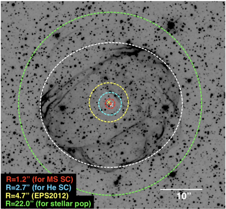
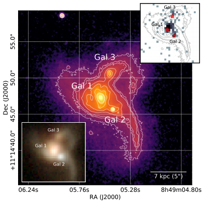
Figure 1: SN 0519–69.0. The authors fit the SN shell in Hα (taken by HST) to an ellipse marked in white, with the white cross at its center. Averaging this with the center determined by another publication, the authors take the red ‘x’ as the explosion center. The red dashed circle marks the runaway distance for a MS companion (0.2 pc) and the cyan circle marks this distance for helium companions (0.6 pcs). The green circle denotes the search radius for background stars taken between the cyan and green circles. Similar figures for the other supernovae are available in the paper. [Li et al. 2019]

Searching for a Companion

The authors of today’s paper set out to look for potential companions dancing around SN remnants, the shells of material left over by SN explosions. The sought-after companions, which could be main sequence (MS) stars, red-giant stars, or helium stars, may have lost their outer layers in the deadly explosion but could live on as a dense core. These surviving cores should be identifiable — they probably move differently as a result of the explosion, and they likely look different in color.

Knowing that these companion cores will stand out from background stars, the authors choose three Type Ia supernovae remnants to investigate for survivors: SN 0519–69.0, DEML71, and SN 0548–70.4. Because SN remnants in our own galaxy can be tough to look at through the galactic plane, these remnants are all located in the Large Magellanic Cloud (LMC). The first two SNe on the list have been examined before with no luck, but the authors hope that their new Hubble Space Telescope data will shed new light on these areas of the sky.

Today’s authors use those two methods, analyzing the color and the motion of stars surrounding the chosen SNe to search for surviving companions. Before they can do this though, they need to determine a proper area to search.

Where to Look?

SNe remnants have a generally circular or elliptical shape, as the shock from the explosion propagates outward in all directions and interacts with the interstellar medium. By finding the geometrical center of the remnant’s visible shell, the authors estimate an explosion site (see Figure 1).

If a star survives a SN explosion, its velocity after the supernova should be the sum of its own orbital velocity and the velocity of the progenitor’s translational velocity. Previous studies have determined the maximum speed that a MS or helium star could be traveling after a Type Ia SN. Using these velocities, the authors calculate just how far a companion core could have traveled away from the SN center since the explosion and narrow their search for survivors to this area (called the “runaway distance”). And of course, there has to be a control — the authors determine a set of background stars to which they can compare their potential survivors (see Figures 1 & 2).

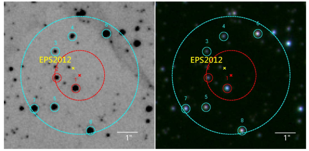
Figure 2: SN 0519–69.0. Stars with V mag < 23.0 (most likely cutoff for potential companions from Schaefer et al. 2012) that lie within the runaway bounds. These are analyzed as potential survivors in the CMDs and RV plots. Red for MS, cyan for helium stars. [Li et al. 2019]

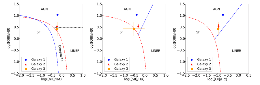
Method 1: Examining Color

To examine the color of their potential survivors, the authors plot the stars’ colors and absolute magnitudes on a very useful diagram called a color–magnitude diagram (clever name, right?). Included on these plots are all the candidate companions and background stars, as well as several “post-impact evolutionary tracks” (see Figure 3). These tracks are merely paths on the diagram that show how a MS or helium companion star, after a SN explosion, should change in color (which depends on its temperature) and brightness according to its initial mass. Therefore, if there are any true surviving companions, they should lie on these tracks.

You may have noticed that red-giant stars, although a potential type of companion, have not been included in the search up to this point. Astronomers do not yet have evolutionary tracks for red giants, unfortunately. More on why that is unfortunate in just a second.

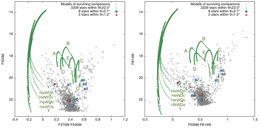
Figure 3: CMDs for SN 0519–69.0. Left: The HST equivalent of a V vs B–V CMD. Right: The HST equivalent of an I vs V-I CMD. Evolutionary tracks are shown in green, with the helium star tracks situated in the left of each diagram. [Li et al. 2019]

Method 2: Examining Motion

The second method for identifying surviving companions is to examine their radial velocity (RV), the speed of their motion away from or towards the Earth. Astronomers need spectral data to get this, which the authors only have for SN 0519–69.0 and DEML71. Now, although we don’t have a great idea of what that RV should be, it clearly should be different from the RV of background stars not involved in the SNe. The authors look at the distributions of RVs for relevant stars (candidates or candidates+background — Figure 4) to determine which stars have abnormal RVs, and these are considered candidate survivors.

Results

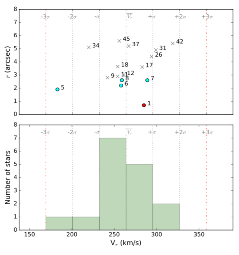
Figure 4: RV for stars with V mag < 21.6 (limiting magnitude for reliable spectral fits). For SN 0519–69.0, there were only a few candidates, so the authors included the background stars to establish a distribution. Star #5 is the strange one — it is not moving with the rest of the group! Again, the same figures for the other SNe are available in the paper. [Li et al. 2019]

So what came of this survivor search? Let’s take a look at each supernova.

SN 0519-69.0: The CMD search did not return any potential companions. The stars within the runaway radii have colors that do not fall on one of the corresponding evolutionary tracks. However, there is a star with a strange (> 2.5σ away from the mean) RV, as shown in Figure 4. This oddball star may be considered a candidate if it also fell on the evolutionary tracks, but it does not. Why, you ask? Well, it seems that this star is likely a red giant, as it falls on the red giant branch in the CMDs. So, this star could very well be a candidate, but red-giant evolutionary tracks must be developed for the authors to confirm either way (that’s the unfortunate part).

DEML71: This SN has a very similar story to SN 0519-69.0. No stars can be considered candidates from the CMDs, but there is indeed a star with a strange RV. However, as we saw before, it seems to be a red giant and therefore cannot be considered a candidate due to the lack of theoretical data. Boo.

SN 0548-70.4: Inspection of the CMDs show that there is indeed a star that falls on one of the MS evolutionary tracks! Great! … But wait… there’s more. This star does not appear on evolutionary tracks for both colors, so the authors remain skeptical — a true candidate should fall on tracks for both CMDs. Furthermore, the part of the evolutionary track that the candidate does fall on indicates an age of only ~110 years. This SN remnant is about 10,000 years old, so obviously this star is unrelated to the explosion and is likely not the candidate the authors were looking for.

As with all science, null results are still results. Even though no surviving cores were identified, the authors still gained valuable information — like, we really need some red-giant post-impact evolutionary tracks. Or perhaps these SNe are not what they seem; if the SD and DD models are drastic oversimplifications, then our predictions for them won’t lead us to surviving stars. Many other types of Type 1a supernova have been proposed, such as sub-/super-Chandrasekhar or spin-up/spin-down. All in all, astronomers rely on models quite often, since we can’t go grab a star. With comparison to more models, we will have a better picture of reality.

About the author, Lauren Sgro:

I am a PhD student at the University of Georgia and, as boring as it may sound, I study dust. This includes debris disk stars and other types of strange, dusty star systems. Despite the all-consuming nature of graduate school, I enjoy doing yoga and occasionally hiking up a mountain.

26 November 2019

Not Far in the Dark

Editor’s note: Astrobites is a graduate-student-run organization that digests astrophysical literature for undergraduate students. As part of the partnership between the AAS and astrobites, we occasionally repost astrobites content here at AAS Nova. We hope you enjoy this post from astrobites; the original can be viewed at astrobites.org.

Title: A Tip of the Red Giant Branch Distance to the Dark Matter Deficient Galaxy NGC 1052–DF4 from Deep Hubble Space Telescope Data
Authors: Shany Danieli et al.
First Author’s Institution: Yale University
Status: Submitted to ApJL

At the end of March last year, the Dragonfly team announced the discovery that galaxy NGC 1052–DF2 had almost no dark matter (see this Astrobite for more on the discovery). This announcement set off a flurry of responses, since the existence of an object like NGC 1052–DF2 has enormous implications for models of galaxy formation and behavior (see this Astrobite for a great summary of some of the initial responses).

Figure 1: A color–magnitude diagram of globular cluster Messier 55 (M55). The TRGB can be seen at the upper right. [B.J. Mochejska, J. Kaluzny (CAMK), 1m Swope Telescope]

To determine how much dark matter a galaxy has, you have to compare its stellar mass (which comes from estimating how many stars it has) and its dynamical mass (which comes from measuring how the contents of a galaxy are moving). Measurements of stellar mass and dynamical mass are extremely dependent on distance, which was the basis of some criticisms of the NGC 1052–DF2 discovery paper.

Tip of the Red Giant Branch (TRGB) stars (see Figure 1) are stars that have just run out of hydrogen and started to burn helium. Being at this turning point in their lives gives TRGB stars a characteristic brightness and color, meaning that they can be used to measure distances (like here). In today’s paper, members of the Dragonfly team use TRGB stars to measure the distance to NGC 1052–DF4, another seemingly dark-matter-deficient galaxy.

Tipped Off (by) the Edge

The authors base their study on observations taken by the Hubble Space Telescope (see the cover image above). To identify the TRGB stars, the authors first separate out RGB stars from the rest. They then group these RGB stars based on their brightness to get a luminosity function for the galaxy. The first derivative of the luminosity function is then used to identify the location of the TRGB stars (see Figure 2). This technique is called edge detection.

The identified location of the TRGB doesn’t seem to shift too much with radius, and pegs the apparent magnitude of TRGB stars (in the I₈₁₄ band) at 27.25 ± 0.11 mag. The absolute magnitude of TRGB stars in the I₈₁₄ band is about -4.0 mag. Taken with the apparent magnitude and median color of the identified TRGB stars, this gives a distance of 18.3 ± 1.0 megaparsecs (1 megaparsec is ~3.26 million light years) to NGC 1052–DF4.

Figure 2. Color–magnitude diagram (CMD) of RGB stars in NGC 1052–DF4 (left), the luminosity function of the galaxy (middle), and the output of the edge detection algorithm (right). The gray points and black points in the CMD are the stars that were rejected and accepted respectively, following quality cuts. [Danieli et al. 2019]

Not So Distant

To understand and account for photometric errors (which edge detection is unable to do), the authors inject artificial stars into their observations and recover them. The authors then re-estimate the galaxy distance by modeling the galaxy using parameters obtained from their observations. They get a TRGB apparent magnitude of 27.31 ± 0.03 ± 0.09 (the first error spans the central 68% of the magnitude likelihood and the second error comes from systematic uncertainty) and a distance of 18.8 ± 0.9 megaparsecs.

The distance to NGC 1052–DF4 the authors obtain agrees with the distance obtained via surface brightness fluctuations (how the brightness of a galaxy varies if you divided it into segments and compared them). However, their TRGB distance differs by varying degrees from TRGB distances obtained by other studies. The authors suggest that this might be due to non-TRGB stars being mistaken for TRGB stars.

The TRGB distance obtained in this work places NGC 1052–DF4 in close proximity to NGC 1052 and NGC 1052–DF2, consistent with previous measurements. It also supports the interpretation that NGC 1052–DF4 is a dark-matter-deficient galaxy. NGC 1052–DF2 will receive similar treatment very soon, continuing the fascinating story of these strange galaxies.

About the author, Tarini Konchady:

I’m a third-year graduate student at Texas A&M University. Currently I’m looking for Mira variables in optical to help calibrate the extragalctic distance ladder. I’m also looking for somewhere to hide my excess yarn and crochet hooks (I’m told I may have a problem).

19 November 2019

The Slowly Cooling White Dwarfs Who Say Ne!

Editor’s note: Astrobites is a graduate-student-run organization that digests astrophysical literature for undergraduate students. As part of the partnership between the AAS and astrobites, we occasionally repost astrobites content here at AAS Nova. We hope you enjoy this post from astrobites; the original can be viewed at astrobites.org.

Title: A Cooling Anomaly of High-Mass White Dwarfs
Authors: Sihao Cheng (程思浩), Jeffrey D. Cummings, and Brice Ménard
First Author’s Institution: The Johns Hopkins University
Status: Accepted to ApJ

The European Space Agency’s Gaia mission has revolutionized astronomy, and it will continue to do so as its mission progresses. Pristine color–magnitude (or Hertzsprung-Russell) diagrams can be made with the extremely precise distances the mission provides, uncovering new features. Today’s paper focuses on explaining some interesting features discovered in the white dwarf sequence seen in Gaia’s second data release (GDR2).

White dwarfs are the end state of most stars. After evolving off the main sequence, low mass stars shed their outer layers, leaving behind an extremely hot core of (in most cases) carbon and oxygen. At this point, the white dwarf will cool off forever. GDR2 revealed some interesting structure in this cooling sequence, including evidence of double white dwarf mergers and a splitting of hydrogen-atmosphere white dwarfs (“DAs”, in the A branch) from those with helium atmospheres (“DBs”, in the B branch). In this context, a branch is a concentration of stars off of the main sequence that stars evolve along or through. A third and less understood branch was found to contain “DQ” white dwarfs, which show carbon in their atmospheres; this was named the Q branch. The GDR2 white dwarf cooling sequence is shown in Figure 1.

Figure 1: The HR diagram of white dwarfs selected from GDR2 for this work. Model ages and masses are indicated by dashed lines. Color indicates the velocity of each star. The Q branch is indicated by the red arrow in the inset and outlined in the main figure. [Cheng et al. 2019]

This Q branch is not aligned with the lines of constant age or mass, indicating that it is not an overdensity in a certain type of white dwarf, but is instead caused by a delay in cooling. Further evidence of the cooling-delay hypothesis is given by the velocity dispersion of stars in the sequence. As stars age there is an increasing probability of gravitational interactions with other stars. These interactions “stir” the stars and increase their velocities with respect to the average movement of stars at a given location in the galaxy. As shown in Figure 1, there is a clear excess of high transverse velocity stars (pink dots) in the Q branch, indicating that they are actually much older than would be predicted by their position on the HR diagram. Interestingly, the stars in the “late” branch in Figure 1 are lower velocity, yet cooler, than those in the Q branch, indicating that there is likely more than one population of stars: one that has a delay in cooling and one that does not.

To test this hypothesis, the authors ran a statistical model of white dwarf evolution. The model includes double white dwarf mergers (which also produce a discrepancy between velocity photometric ages), tracks the ages and velocities of the stars, and tries to match the observations. The parameters of interest for the cooling hypothesis are the fraction of stars that undergo a cooling delay and the length of that delay. After examining many other parameters (see section 4 of the paper for all the gory details), the authors show that 6% of high-mass white dwarfs appear to experience an 8-billion-year delay of cooling as they evolve along the Q branch. Since this delay causes a pile-up, about half of white dwarfs on the Q branch are delayed. The authors also constrain the double-white dwarf merger fraction to about 22% of massive white dwarfs. Figure 2 shows the HR diagram produced by the simulation.

Figure 2: HR diagram showing the two populations of white dwarfs evolving down the cooling sequence over time. Each second corresponds to 1 Gyr. [Sihao Cheng et al.]

The authors propose that ²²Ne settling could be the source of the cooling delay. Since the gravity of white dwarfs is so strong, heavy elements sink toward the core, releasing gravitational energy in the process. This energy release slows cooling. The authors calculate that the temperature regime where this settling occurs, shown in Figure 3, matches the position and shape of the Q branch. The delay length is also roughly consistent with the amount of energy that would be released, although more work is needed here.

Figure 3: The effective zone of ²²Ne settling for two different abundances of ²²Ne. The cooling delay happens when the luminosity of ²²Ne settling is similar to the surface luminosity. This region is narrow and matches the position and shape of the Q branch quite well. [Cheng et al. 2019]

While the author’s statistical cooling delay model can replicate the observations, more work must be done to confirm if the proposed physical mechanism, ²²Ne settling, is the true cause of the cooling delay. Specifically, this process must be incorporated into cooling models of massive white dwarfs. Gaia’s precision measurements and extremely large sample size continue to raise interesting questions and help us answer them. The bunch-up of white dwarfs examined in this paper would not be visible in a smaller or noisier sample of stars, demonstrating the wealth of knowledge that Gaia is capable of unlocking after only about half of its mission.

About the author, Samuel Factor:

Sam Factor is a 5th year Ph.D. candidate at The University of Texas at Austin studying direct imaging of extrasolar planets and low mass binary stars. He uses an interferometric post processing technique to allow the detection of companions below the diffraction limit of the telescope.

12 November 2019

A Discovery of a Triple AGN System

Editor’s note: Astrobites is a graduate-student-run organization that digests astrophysical literature for undergraduate students. As part of the partnership between the AAS and astrobites, we occasionally repost astrobites content here at AAS Nova. We hope you enjoy this post from astrobites; the original can be viewed at astrobites.org.

Title: A Triple AGN in a Mid-Infrared Selected Late Stage Galaxy Merger
Authors: Ryan W. Pfeifle, Shobita Satyapal, Christina Manzano-King, Jenna Cann, et al.
First Author’s Institution: George Mason University
Status: Published in ApJ

What Are AGN and Why Do I Care?

An AGN, or active galactic nucleus, is the epitome of a fascinating and truly awesome astrophysical object. An AGN consists of a black hole that happens to be surrounded by gas and dust that is close enough to form an accretion disk and fall into the black hole. As a result, the black hole (now AGN) forms these enormous, extremely bright, and hottt jets. AGNs are quite useful for those interested in learning more about black holes (who isn’t?), but black holes on their own don’t emit any sort of radiation. It’s only when they come in contact with or are in front of other, directly detectable things that we can then indirectly learn about these incredible astrophysical phenomena.

Artist’s impression of an active galactic nucleus sporting a relativistic jet. [ESO/M. Kornmesser]

Astronomers are particularly interested in supermassive black holes, which seem to be in the center of the vast majority of galaxies. Supermassive black holes also seem to co-evolve with their host galaxy, at least according to the most popular theory of cosmology: ΛCDM. It’s quite interesting to think that a single supermassive black hole in the center of the galaxy, while very massive for a single object, could also potentially govern the evolution of its much larger and more massive entire host galaxy. For example, the supermassive black hole in the center of the Milky Way is about 3 million solar masses and just about a light-minute in diameter — but compare that to the Milky Way itself, which is 150 billion solar masses and over 50,000 light-years wide. How could that relatively small black hole have such an impact on an entire galaxy?

Since AGNs are super bright, astronomers can detect them from very far away. This allows us to explore how supermassive black holes affect galaxy evolution across cosmic time. AGNs only exist where there is an excess amount of dust and gas in a galaxy. Nowadays, when we look at nearby galaxies, they are lacking in dust and gas compared to galaxies at a redshift of z = 2. Examining galaxies at a redshift of z = 2 mean that we are looking back to a time when the universe was only about a quarter of its current age. Back then, galaxies contained a TON of gas and dust that was used for star formation — and also as fuel for AGNs. This redshift is therefore a key time period that astronomers can probe to better understand how galaxies and their active supermassive black holes evolve to what they are today.

Where Does the Triple AGN Come In?

One of the main drivers of galaxy evolution is galaxy mergers. The math is simple: galaxy + galaxy = bigger galaxy. When two galaxies collide, the stars inside of them don’t run into each other, but the gas and dust in each galaxy do collide and interact, producing starburst events and, you guessed it, powering AGNs! So if we wanted to hunt down some AGNs, mergers are a fantastic place to start.

Artist’s illustration of an active galactic nucleus shrouded by gas and dust. [NASA/JPL-Caltech]

Cosmological simulations predict that ~16% of all mergers actually contain three galaxies — a triple merger. This offers up the possibility of a triple merging system where each of the galaxies involved in the collision has an active galactic nucleus. If we believe our modern theory of the universe (ΛCDM), triple AGN systems must exist, but since there is going to be a lot of dust in the system, they could be obscured behind thick sheets of dust. This possible obscuration — plus their relative rarity — makes these systems difficult to detect. Today’s paper offers up a proposed detection of such an object.

The Detection of a Triple AGN

Detecting AGN is not always straightforward. The signals that AGNs produce are similar to other high-energy phenomena in the universe, so in order to be absolutely sure you have detected an AGN, you need to use the full electromagnetic spectrum. AGN flux peaks at X-ray wavelengths, so you definitely want to use the Chandra and NuStar observatories. AGNs also have a specific optical signature to look out for, so you can use a big ol’ optical telescope like the Large Binocular Telescope, and optical surveys like SDSS. And due to the dust surrounding the AGN, its original emission will be reddened, and even the dust itself can be visible in infrared wavelengths. Today’s paper utilized telescopes that operate in each of these wavelengths to confirm a triple AGN system: SDSS J0849+1114. (Radio is also useful, and the authors say that they are working on another paper that will include the radio data).

Figure 1: This figure shows the triple merger system: three galaxies, each of which host an AGN. The middle image is from the Hubble Space Telescope (infrared); the image in the upper right is from Chandra (X-ray); and the lower left is from SDSS (optical). [Pfeifle et al. 2019]

To validate their claim of an AGN system, this paper also explored some other possible explanations for each of their detections, and ruled each of them out. One alternate explanation is star formation. I mentioned that at around the same time AGNs become active, star formation is also very active. Could star formation explain the X-ray emission this paper reports? To answer this, the authors turned to their optical data. Using spectral lines specific to star formation signatures, they were able to calculate the star formation rate needed to explain the optical emission they receive. Then, using that rate, they calculated how much X-ray emission would be expected — and it’s an order of magnitude (10x) lower than what they see in X-rays. Okay, so star formation won’t cut it. What about ionized shocks? A shock can be produced by a sudden change in pressure, usually associated with supernova. They are bright and high energy; could that be causing the X-ray signature they see? It could explain both the X-ray and optical luminosity they receive, however, the optical spectroscopy is missing some signatures that would be present if there were shocks. Plus, it would be super rare for three shocks to coincidentally happen near the center of each galaxy.

Figure 2: These plots show the line ratios of various elements. That basically means that we measure the emission we get at wavelengths that correspond to very specific atomic transitions. We can use that emission, and ratios of emission from different elements, to determine what kind of environment we are looking at. In these specific plots, the blue, red, and yellow shapes represent the centers of the three galaxies, and the markers can either lie in the AGN, SF (star formation), or LINER (low-ionisation nuclear emission-line region) category. We see here that the three line ratios that they explore suggest that each of the galaxies contain AGN. [Pfeifle et al. 2019]

Given the X-ray, optical, and infrared data of this system, this paper concludes with some certainty that they have discovered a triple AGN system. This triple AGN system surely will receive more follow-up study, and the obvious next step is to search for more systems like it! This triple AGN detection is so special because it is predicted by ΛCDM cosmology, and it has the added bonus of offering a possible solution to the final parsec problem. Hopefully, with a handful of known triple AGN, we can start to better test our current theories of physics that govern the universe.

About the author, Jenny Calahan:

Hi! I am a second year graduate student at the University of Michigan. I study protoplanetary disk environments and astrochemistry, which set the stage for planet formation. Outside of astronomy, I love to sing (I’m a soprano I), I enjoy crafting, and I love to travel and explore new places. Check out my website: https://sites.google.com/umich.edu/jcalahan

5 November 2019

Ancient Aurorae: Assyrian and Babylonian Astrologers Recorded the Oldest-Known Solar Storms

Editor’s note: Astrobites is a graduate-student-run organization that digests astrophysical literature for undergraduate students. As part of the partnership between the AAS and astrobites, we occasionally repost astrobites content here at AAS Nova. We hope you enjoy this post from astrobites; the original can be viewed at astrobites.org.

Title: The Earliest Candidates of Auroral Observations in Assyrian Astrological Reports: Insights on Solar Activity around 660 BCE
Authors: Hisashi Hayakawa, Yasuyuki Mitsuma, Yusuke Ebihara and Fusa Miyake
First Author’s Institution: Osaka University, Japan
Status: Published in ApJL

Humans have always been star-gazers. Since time immemorial we have looked to the heavens and tried to make sense of what we saw there. Thousands of years ago the motions of heavenly bodies and the appearances of comets and meteors were believed to be omens that determined the fates of kings and predicted the downfall of empires. Official court astrologers were employed to read these portents in the sky and divine their (hopefully favourable) meanings.

Many of these ancient observations of celestial events still survive as written records in the form of cuneiform tablets inscribed over two millennia ago. Cuneiform was one of the earliest systems of writing and was typically inscribed on rectangular clay tablets using a blunt reed to produce wedge-shaped marks. Cuneiform tablets have been discovered at archaeological sites all across the Near and Middle East, such as at the ancient Assyrian city of Ninevah (modern-day northern Iraq) — once the largest city in the world. They were used for almost everything, including recording celestial events, documenting laws and religious beliefs, and even for entire literary works — such as the famous Epic of Gilgamesh.

Figure 1: Y. Mitsuma’s tracings of the photographs of cuneiform tablets taken by H. Hayakawa. These cuneiform tablets are preserved in the British Museum. [Mitsuma et al. 2019]

Today’s astronomers track changes in the Sun’s activity using a variety of methods, including examining the occurrence rates of sunspots. Sunspots are associated with solar flares and coronal mass ejections — huge eruptions composed of high-energy protons and electrons that can cause geomagnetic storms when they are directed towards the Earth. A well-known feature associated with particularly strong geomagnetic storms is the occurrence of aurorae, produced when high-energy particles excite atoms in the Earth’s atmosphere. Astronomers have been observing sunspots ever since the advent of the telescope, but if we want to examine the history of the Sun’s activity prior to this we need to turn to historical records of phenomena linked to solar activity, such as aurorae.

A team led by Hisashi Hayakawa, a researcher at Osaka University and the lead author of today’s paper, carried out a survey of tablets dating from the 8th and 7th centuries B.C. looking for references to aurorae, that might match evidence inferred from tree ring samples. Tree rings store information on the environmental conditions present at the time of their formation — and during periods of strong solar activity, they show enhanced concentrations of the radioactive isotope carbon-14, produced when high-energy particles interact with nitrogen atoms in the atmosphere. Studies of tree-ring samples from around 660 B.C. have been shown to contain elevated carbon-14 levels, and the researchers wondered if they could find any historical references to match this inferred spike in solar activity.

Aurora during a geomagnetic storm that was most likely caused by a coronal mass ejection, taken from the International Space Station. [ISS Expedition 23 crew]

The team found three separate Assyrian and Babylonian cuneiform tablets held in the British museum that referred to “red clouds” and a “red glow” lighting up the night sky and that date from the period 679 to 655 B.C. These descriptions are similar to the previously oldest-known reference to an aurora, found in a Babylonian tablet dating to 587 B.C. The researchers suggest that these descriptions probably refer to a type of auroral activity known as stable auroral red arcs, which are produced by the interaction of strong magnetic fields and the electrons in oxygen atoms.

Although we typically think of aurorae as being a northern-latitude (or southern in the case of the Aurora Australis) phenomenon, this has not always been true. Over time the Earth’s geomagnetic poles shift due to changes in the Earth’s magnetic field, and thousands of years ago the north pole would have been located much closer to the Middle East. Furthermore, strong solar activity, such as coronal mass ejections, can cause aurorae to become visible at much more southernly latitudes. It is therefore quite likely that aurorae would have been visible in the region of these observations during this time period.

These findings constitute the oldest-known written evidence of candidate aurorae and potentially extend the history of the Sun’s activity nearly a century beyond previous records. They could also help us to predict future solar storms, which have the capability of interrupting sensitive electronics on Earth and damaging satellites and spacecraft.

About the author, Jamie Wilson:

Jamie is a graduate student at the Astrophysics Research Centre at Queen’s University Belfast.

1 November 2019

Not All Black Holes That Wander Are Lost

Editor’s note: Astrobites is a graduate-student-run organization that digests astrophysical literature for undergraduate students. As part of the partnership between the AAS and astrobites, we occasionally repost astrobites content here at AAS Nova. We hope you enjoy this post from astrobites; the original can be viewed at astrobites.org.

Title: A New Sample of (Wandering) Massive Black Holes in Dwarf Galaxies from High Resolution Radio Observations
Authors: Amy Reines, James Condon, Jeremy Darling, Jenny Greene
First Author’s Institution: Montana State University
Status: Accepted to ApJ

Hubble image of UGC 5497, an example of a dwarf galaxy. Do these small galaxies also host massive black holes at their centers? [ESA/NASA]

At the centre of the most massive galaxies resides a supermassive black hole around which everything rotates. Typically, these black holes are identified by measuring the velocity and shape of the orbits of a galaxy’s innermost stars as they rotate around its centre. However, this approach is less effective when we consider much lighter galaxies like dwarf galaxies. These galaxies are much fainter than their high mass counterparts so their stellar populations can’t be sufficiently resolved by current missions. Instead, a lot of recent work in the field focuses on identifying the energetic process a massive black hole undergoes when it accretes gas and dust, turning the central region of a galaxy into an active galactic nucleus (AGN). By identifying the incidence of AGN, a lower limit on the distribution of black holes in dwarf galaxies can be obtained. Today’s authors adopt this approach to further study their black hole population and produce some surprising results.

Constructing the Sample

AGN emit across the electromagnetic spectrum, but today’s authors decide to use centimetre radio emission, as they argue it isn’t as strongly extinguished by galactic dust. An initial sample of 43,707 dwarf galaxies were identified in the NASA-Sloan Atlas. To maximise the number of AGN detections, the authors first matched this dwarf galaxy sample to archive data from the Very Large Array (VLA). 111 matches were found in the VLA “Faint Image of the Radio Sky at Twenty Centimeters” survey within 5 arcseconds of the galaxy’s optical centre. These 111 objects were re-observed by the VLA in the A-configuration. In this configuration, the antenna dishes are spread out as widely as possible along each arm of the Y-shape to create a dish with an effective diameter of 22 miles; this allows the authors to take full advantage of the VLA’s high spatial resolution. From this, they were left with 35 dwarf galaxies containing 44 significant compact radio sources.

Accounting for Stellar Birth and Death

AGN are not the only objects that can produce compact and intense radio emission; this emission could also point to the births and deaths of stars. Before they could attribute these compact radio sources to AGN, the authors tried to remove the possibility of a stellar origin for the emission.

Areas of a galaxy where large amounts of star formation have taken place, known as HII regions, are dominated by ionised atomic hydrogen. These regions are typically identified by looking for signs of Bremsstrahlung (or braking radiation), emitted when a free electron is slowed down by interaction with the copious amounts of ionised hydrogen present. The authors model the observed compact radio emission as if produced by this process, from which they calculated a thermal star formation rate. Each galaxy also has a star formation rate taken from the NASA-Sloan Atlas, calculated using the dust-corrected ultraviolet light from the whole galaxy. The dark blue and red points in the left-hand panel of Figure 1 highlight the 20 radio sources found to have thermal star formation rates that are much larger than the star formation rates from the NASA-Sloan Atlas. It doesn’t make sense for a subsection of a galaxy to be producing more stars than are being produced in the whole of the galaxy, so the authors can rule out star formation causing emission observed in these 20 radio sources.

Figure 1: Investigating alternative sources of the observed radio emission in each galaxy. The left-hand panel compares the star formation rate from the galaxy as a whole to that predicted by assuming all the radio emission is from Bremsstrahlung. Any object falling below the dashed line is considered to have emission consistent with star-formation; W49 A is a highly star-forming region of the Milky Way included as a comparison. The right-hand panel compares the expected emission from a population of supernovae to the observed emission. The dashed line describes the supernova luminosity function, with the solid lines describing observed luminosities three times brighter and dimmer than the function. Any object below the upper solid line is considered to have radio emission consistent with supernovae emission. [Reines et al. 2019]

Similarly, stars at the end of their lives — supernovae — also produce large amounts of radio emission. To model this emission the authors make use of a supernova luminosity function that describes the predicted supernovae luminosity as a function of the host galaxy’s star formation rate and the observed radio luminosity, shown as a dashed line in the right-hand panel of Figure 1. For each galaxy, the supernova luminosity function is integrated across the full range of possible supernova luminosities and compared to the observed radio luminosities. In the right-hand panel of Figure 1, we again see the emission from these same 20 compact radio sources in the upper left region. This shows, for these 20 radio sources, the observed emission is at least 3 times as bright as the expectation from supernovae emission, so the authors can rule out supernovae causing emission observed in these 20 radio sources as well.

Wandering Black Holes

Since the emission from these 20 radio sources cannot be explained by star formation or supernovae, the authors conclude that they are AGN. Figure 2 shows the positions of 13 of these AGN as red crosses within their dwarf galaxy host. The high spatial resolution of the radio measurement highlights the really interesting result of today’s paper: a number of these AGN are seen well outside the approximate optical galactic centre, indicated by the white circle. Recent simulations predict that roughly half of all massive black holes are expected to be found in the outskirts of their host galaxy. It is believed off-nuclear black holes, such as these, could have been recently stripped from a neighbouring galaxy the host recently interacted with, or perhaps we are seeing the gravitational recoil from two recently merged black holes.

Figure 2: Images of the 13 dwarf galaxies in Sample A believed to host radio-selected AGN. The red cross indicates the very secure radio AGN position; the white circle indicates the region measured by the SDSS, thus the galaxy’s approximate optical centre. Only these objects are shown as the remaining 7 objects in Sample B did not have a second measurement of mass or redshift from the VLA radio measurement thus the authors were unsure whether to consider them dwarf galaxies. [Reines et al. 2019]

Detections of AGN, and the black holes powering them, are still rare in dwarf galaxies compared to the near ubiquity identified in high-mass galaxies. Any additional detections are crucial to furthering our understanding of the true distribution of black holes in dwarf galaxies. Where today’s paper has excelled, though, is by exploiting the high spatial resolution of the VLA to identify a population of black holes outside the centres of their host galaxies. Not only is this a surprising observational result, but it represents one of the first confirmations of simulations that suggest these massive black holes tend to wander the outskirts of their host galaxies.

About the author, Keir Birchall:

Keir is a PhD student at University of Leicester studying methods to identify active galactic nuclei in various populations of galaxies to see what affects their incidence. When not doing science, he can be found behind the lens of a film camera or listening to the strangest music possible.

30 October 2019

Plenty of Gas Left in Giant Dead Disk Galaxies

Editor’s note: Astrobites is a graduate-student-run organization that digests astrophysical literature for undergraduate students. As part of the partnership between the AAS and astrobites, we occasionally repost astrobites content here at AAS Nova. We hope you enjoy this post from astrobites; the original can be viewed at astrobites.org.

Title: Nearly all Massive Quiescent Disk Galaxies have a Surprisingly Large Atomic Gas Reservoir
Authors: C. Zhang et al.
First Author’s Institution: Peking University, China
Status: Published in ApJL

A concept fundamental in astronomy is that stars form from cold, dense molecular gas clouds. Applied to the formation and evolution of galaxies, star-formation is understood as being directly supported by an abundance of this cold molecular gas. We find that in star-forming galaxies — typically disk-like with blue spiral arms — there is a large reservoir of this cold molecular gas from which rapid star-formation can be sustained. Quiescent galaxies, on the other hand — typically elliptical-like with red colors — do not actively form stars. Hence, they have been long thought to have only a scarce supply of cold molecular gas, likely as a result of either vigorous star-formation in the past, some sort of gas reservoir removal event, or a combination of the two.

There is overwhelming evidence that star-forming and quiescent galaxies inhabit very different environments in our universe. While star-forming galaxies are generally found alone or in small groups, quiescent galaxies are often found residing in large galaxy clusters with tens to hundreds of cluster members. This so-called morphology-density relation tells us something fundamental about the role of environment in shaping galaxy properties. In particular, it suggests that the cluster environment influences the ceasing (or quenching) of star-formation.

Figure 1. Archetypal quiescent elliptical galaxies (left) and star-forming spirals (middle) comprise the vast majority of galaxy demographics. Rare and poorly understood red disk spirals remain a puzzling mystery (right). [Masters et al. 2010]

The largest and most massive galaxies typically reside near the center of a cluster. We label them “central” galaxies to contrast them with smaller “satellite” galaxies that reside in the cluster outskirts. Most massive central galaxies are quiescent. One mechanism that has been proposed to explain this cessation of star formation in these particularly massive central galaxies is so-called hot-halo quenching. In this scenario, a massive central galaxy is kept from refreshing its supply of cold molecular gas from its surroundings because the immense gravitational force experienced by the gas as it enters the halo of the central galaxy is so great that it becomes shock heated. Although still accreted into the central galaxy, the now-hot gas becomes unsuitable to form stars.

Today’s paper discusses new and surprising findings about the gas content of these massive central galaxies, and how the galaxies are kept from forming stars.

A statistically large sample of nearby massive central galaxies was carefully selected from the Sloan Digital Sky Survey (SDSS). Instead of focusing on just typical giant central galaxies that have elliptical morphologies, the authors chose to examine the ellipticals side-by-side with little-appreciated massive central disk galaxies. These kinds of galaxy cross-breeds are extremely rare, but potentially interesting objects for understanding the complex and poorly understood mechanisms that drive star-formation cessation. Morphological classifications of elliptical and disk galaxies were taken from the citizen science project Galaxy Zoo, which crowd-sources galaxy classification through an online web platform accessible to anyone.

However, the SDSS data is only half the story. The SDSS galaxies were crossed matched with deep centimeter-wavelength surveys (ALFALFA and GASS) in order to obtain measurements of the atomic gas (H I) in these galaxies. While the atomic gas is too hot to directly form stars, given the right conditions it may cool down into molecular gas (H₂).

Figure 2. (Left) the distribution of massive elliptical and disk central galaxies, with the fractional abundance of disk galaxies shown in grey. (Middle) the strength of H I detection as a function of star-formation rate for disk and elliptical central galaxies. (Right) Similarly, the atomic gas mass. [Zhang et al. 2019]

The study reports a surprising finding: nearly all massive central disk galaxies have exceedingly large atomic gas reservoirs, especially when compared to those of ellipticals, as shown in Figure 2. Not only this, but massive disk galaxies with high star-formation rates have almost the same atomic gas mass compared to those with lower star-formation rates. In other words, massive quiescent central disk galaxies are as abundant in atomic gas as star-forming ones.

Importantly, this implies that massive quiescent central disk galaxies do indeed have the raw gas supply necessary to form stars. The lack of star formation then must either be due to a marked inefficiency in converting atomic gas into molecular gas, difficulty in forming stars from the molecular gas, or both.

Figure 3. Atomic (red) and molecular (blue) gas mass as a function of star-formation rate in massive central disk galaxies. [Zhang et al. 2019]

A complementary investigation of the cold molecular gas content of these massive central disk galaxies with the COLD GASS survey suggests that reservoirs of cold molecular gas are, unsurprisingly, significantly smaller for central disk galaxies with low star-formation rates, and vice versa. While this is consistent with our current picture of star formation, it contrasts sharply with the related finding that atomic gas mass does not change with star-formation rate, as shown in Figure 3.

Taken together, this investigation into the gas content of massive central disk galaxies illustrates that although their atomic gas content is universally large compared to central ellipticals, their star-formation cessation is still driven by a dearth of cold molecular gas. Yet, the precise mechanism keeping the atomic gas from eventually giving way to star formation remains elusive.

About the author, John Weaver:

I am a second year PhD student at the Cosmic Dawn Center at the University of Copenhagen, where I study the formation and evolution of galaxies across cosmic time with incredibly deep observations in the optical and infrared. I got my start at a little planetarium, and I’ve been doing lots of public outreach and citizen science ever since.

29 October 2019

A Second Mysterious Radio Outburst from Magnetar XTE J1810-197

Editor’s note: Astrobites is a graduate-student-run organization that digests astrophysical literature for undergraduate students. As part of the partnership between the AAS and astrobites, we occasionally repost astrobites content here at AAS Nova. We hope you enjoy this post from astrobites; the original can be viewed at astrobites.org.

Title: Distinct properties of the radio burst emission from the magnetar XTE J1810−197
Authors: Y. Maan, B.C. Joshi, M. Surnis, M. Bagchi, P. K. Manoharan
First Author’s Institution: ASTRON (Netherlands Institute for Radio Astronomy)
Status: Published in ApJL

Pulsars. Fast Radio Bursts. Magnetars. The world of high-energy stellar astrophysics has no shortage of weird objects that do not always behave like we think they should. From the mysterious workings inside a neutron star to the unknown reason behind why some fast radio bursts repeat, these sources continue to surprise and mystify us. Now, the world of magnetars, stars with incredibly high magnetic fields, just got a little more interesting.

Magnetars: Not Your Average Stellar Objects

Magnetars (short for “magnetic stars”) are neutron stars with some of the strongest magnetic fields in the universe. Their magnetic field strengths are on the order of ~10¹⁵ Gauss; to put this in perspective, the magnetic field of the Earth that shields us from the Sun’s rays and produces auroras is about 0.5 Gauss. If a magnetar was at a distance from Earth equal to that of the Moon, it could strip the information off of all of the credit cards on the planet.

Artist’s illustration of a pulsar, a fast-spinning, magnetised neutron star. [NASA]

In 2006, magnetar XTE J1810-197 (which is also classified as an X-ray pulsar because in addition to having a very strong magnetic field, it intermittently emits X-rays) was found to be emitting radio pulses after a very strong outburst of energy in the radio-frequency regime. At the beginning of this outburst, the pulsar had a nearly flat spectral index. The spectral index tells you how much the total power from the source is dependent on frequency — so if the spectral index was flat, it means that the power emitted was roughly the same at all frequencies. During that burst, radio emission came in spikes that lasted about 10 milliseconds. After the outburst, the source faded in power and essentially turned off before it was re-observed 13 years later and a second radio burst was detected by the authors of today’s work. In Figure 1, you can see how the power emitted by the source declined over time but increased over frequency. Similar “spiky” short-duration radio pulses have been seen in high-energy phenomena such as giant pulses (essentially really bright radio pulses that are occasionally emitted by some sources) and fast radio bursts (FRBs). With these similarities, the bursts from this magnetar could suggest a common origin for these phenomena. Let’s look a bit further into what the authors found from this mysterious source!

What Are These “Spiky” Bursts?

Magnetar XTE J1810-197 was observed by the team in December of 2018 and February of 2019 with the Giant Metrewave Radio Telescope (GMRT) in India. During that time, they found four spiky bursts. When pulsars are observed, we see what is called an average profile, which maps the energy emitted over the time period that the beam crosses our sightline (the pulse phase window) — and we can make similar diagrams for a magnetar. The first panel in Figure 2 shows the regular pulse profile of the magnetar. In their observations, the authors saw that the position of the bursts roughly match that of the average profile. Unlike in the phenomenon of giant pulses, this emission is not confined to a small area of the pulse phase — which differentiates these spiky magnetar bursts from giant pulses. However, these bursts occur on a much shorter timescale than the regular emission, and they occur with different rates at different frequencies, with a width of 1–4 ms at lower frequencies and < 1 ms at higher frequencies (see second panel of Figure 2). Most of these variations are most likely caused by propagation effects in the interstellar medium.

The spectral index of XTE J1810-197’s bursts also seems to vary quite a bit with frequency. Using models of the electron density of the galaxy, the authors calculate that these variations must be intrinsic to the source and not due to the interstellar medium. The variations are also closer to the onset of the outburst, meaning something happens to the spectral index right before a burst happens. This only happens before bursts in earlier sessions, though, not in later observing sessions.

Figure 2: In the left panel, the black line represents the average profile and the blue dashed line shows the average profile from the first observing session of magnetar XTE J1810-197, with the vertical lines showing the different components. In the right panel, the pulse width distributions over time are shown by frequency (B4: 550−750 MHz and B5: 1260−1460 MHz). It is clear that the 550–750 MHz observations show a higher width which can be attributed to scatter-broadening. [Maan et al. 2019]

So What Does All of This Mean?

When magnetar XTE J1810-197’s first burst was observed in 2003, it was found that the radio spectrum was nearly flat, but after the onset of the current outburst, it was found to be much higher. It is possible that the spectrum is higher at lower frequencies. The power emitted by this object has decreased rapidly since the onset of the burst, but there are no clear physical links between spindown rate (how fast the magnetar slows down because it loses rotational energy) and emitted power.

While the outbursts have similarities to some from known objects, it is not quite clear exactly what they are yet. Giant pulses are characterized by an average energy 10 times greater than the average energy emitted by the source. Though the energies are large in the magnetar bursts, they’re not at the limit of giant pulses. The magnetar bursts are actually more similar to the giant micropulses in the Vela pulsar, as the widths are similar, so it is possible that these could be giant micropulses coming from magnetar XTE J1810-197.

Artist’s impression of a fast radio burst observed by the Parkes Radio Telescope. [Swinburne Astronomy Productions]

It has also been suggested by multiple teams that these magnetar pulses could be connected to fast radio bursts. In January, a team led by Astrobites author Aaron Pearlman looked at magnetar J1745-2900, a magnetar that’s very close to the supermassive black hole in the center of our galaxy, and found that the magnetar pulses, just like the FRBs, show frequency structure in single pulses. This was the first time this kind of behavior had ever been observed from a magnetar. The authors of today’s paper found frequency variations of the spiky emission in XTE J1810-197. This spiky emission, which appears in both FRBs and these magnetar pulse, cannot be caused by the interstellar medium. The spikes look similar to the repeating FRB’s pulses, but the long-term frequency drift (essentially when the power emitted is detected at different frequencies) of the FRB’s pulses do not appear in the magnetar’s bursts. Though the magnetar’s brightest burst is ~5x more powerful, the FRB is nearly 10,000 times farther away, implying that it is intrinsically brighter than the magnetar bursts.

The fact that magnetars are the third type of object, after the Crab Pulsar and the repeating FRBs, to exhibit frequency structure in its bursts points to a similar emission mechanism for all three. In addition, the fact that the frequency structure is intrinsic to the star points to some kind of process similar to that of other unexplained high-energy phenomena. What will happen when the star bursts again? Will we find more bursts from other magnetars like this, or repeating FRBs that look similar? Only time will tell!

About the author, Haley Wahl:

I’m a second year grad student at West Virginia University and my main research area is pulsars! I’m currently working with the NANOGrav collaboration (a collaboration which is part of a worldwide effort to detect gravitational waves with pulsars) on polarization calibration. In my set of 45 millisecond pulsars, I’m looking at how the rotation measure (how much the light from the star is rotated by the interstellar medium on its way to us) changes over time, and also looking at other things we can learn from polarimetry. I’m mainly interested in pulsar emission and the weird things we see pulsars do! At WVU, I also work planetarium putting on shows for the public. In addition to doing research, I’m also a huge fan of running, baking, reading, watching movies, and I LOVE dogs!

22 October 2019

Cosmic Archaeology from an Ancient Pulsating Star

Editor’s note: Astrobites is a graduate-student-run organization that digests astrophysical literature for undergraduate students. As part of the partnership between the AAS and astrobites, we occasionally repost astrobites content here at AAS Nova. We hope you enjoy this post from astrobites; the original can be viewed at astrobites.org.

Title: Asteroseismic constraints on the cosmic-time variation of the gravitational constant from an ancient main-sequence star
Authors: Earl Patrick Bellinger, Jørgen Christensen-Dalsgaard
First Author’s Institution: Aarhus University, Denmark
Status: Accepted to ApJL

A Cosmic Constant

The gravitational constant, G, is one of the core fundamental constants of physics, appearing in Newton’s laws of gravitational motion, and therefore in the fundamental theory of gravity. While people historically questioned whether it truly is a constant, Einstein’s theory of general relativity states that G must be constant no matter where in space, or time, you find yourself. However modern work in string theory, which aims to reconcile the theory of gravity with the other fundamental forces of nature, says that the gravitational “constant” can, in fact, vary over extremely long cosmic timescales.

If the gravitational constant was changing in time, we might be able to detect it in systems whose evolution has strongly relied on gravity, such as stars. If gravity was weaker in the past, that would have affected the evolution of a star, changing how it appears today. Measurements of the rate of change of G have been performed in this way using helioseismology, white dwarfs, and globular clusters, as well as studies of the cosmic microwave background. All these experiments draw the same conclusions; that G changes at a completely negligible rate (specifically, by no more than a fraction of a trillionth a year, where the universe is only 13 billion years old).

A Stellar Archaeological Dig

Today’s authors present a new test to more closely approximate the variation of G on truly cosmic timescales. The target of the authors’ study is KIC 7970740, a low-mass, solar-like star on the main sequence that is, most importantly, roughly 11 billion years old! Thanks to high-quality measurements by the Kepler space telescope, this star also has a well measured set of clear stellar pulsations that allow for an asteroseismic analysis, and it is one of the oldest stars for which this is possible.

Because this star is so low-mass, it has had a very relaxed 11-billion-year life on the main sequence, making stellar models of the star relatively simple. This makes it a perfect candidate to study historical changes in the gravitational constant G; if G changed substantially in the the universe’s history, it will have subtly affected the evolution of this star and, as a consequence, the manner in which it pulsates today (see Figures 1 & 2). For example, if G was lower in the past, gravity will have been weaker. As a result, hydrostatic equilibrium will cause the stellar radius to be larger, which increases the star’s energy output (or luminosity). More luminous stars burn faster, changing the composition of the stellar core, which in turn affects how pulsation frequencies appear on the surface.

Modelling the Stellar History

To study the history of G, then, the authors study the history of KIC 7970740, by tweaking the star’s parameters in a stellar model and comparing the result to the observed pulsation frequencies, which are also modelled. Included in these models is a parameter β, representing the fractional change in the gravitational constant, and also the age of the universe, t₀, which are both allowed to vary.

By fitting their evolutionary model to the asteroseismic data (in a process that took 6 months to run!), the authors find a fractional rate of change of G of (2.1 ± 2.9) × 10^-12 yr^-1, or two trillionths a year.

Figure 2: The same as Figure 1, now showing the evolution of the star in terms of two fundamental asteroseismic observables, Δν (the separation between oscillations of different overtones) and δν02 (the separation between oscillations of radial degree 0 and 2). [Bellinger & Christensen-Dalsgaard 2019]

Conclusions

While this result is uncertain, it is in line with previous studies on the change in G from stars — but measured over an extended age range that almost spans the full history of the universe. It is worth noting that the stellar parameters recovered for the star agree with independent studies, indicating that their model fits well and giving additional credibility to these results.

With this result, investigation of G is far from over. With the development of this technique it will become possible to apply it to an ensemble of stars, hopefully yielding a stronger result and/or highlighting any model dependencies that may have affected this result. Continuing this type of research will, hopefully, continue to improve synergies between stellar astrophysics and the most fundamental studies of the universe.

About the author, Oliver Hall:

Oliver is a final year PhD student at the University of Birmingham, UK. He’s a part of their Sun, Stars & Exoplanets research group with a focus on asteroseismology, the study of stellar pulsations, and what it can tell us about stellar populations. When not doing research he enjoys playing piano, hiking, and not moving from the sofa all weekend with a good book, show, or game.

15 October 2019

Building Planets Around a Black Hole

Editor’s note: Astrobites is a graduate-student-run organization that digests astrophysical literature for undergraduate students. As part of the partnership between the AAS and astrobites, we occasionally repost astrobites content here at AAS Nova. We hope you enjoy this post from astrobites; the original can be viewed at astrobites.org.

Title: Planet Formation Around Super Massive Black Holes in the Active Galactic Nuclei
Authors: Keiichi Wada, Yusuke Tsukamoto, and Eiichiro Kokubo
First Author’s Institution: Kagoshima University, Japan
Status: Accepted to ApJ

Nearly 400 years ago, it was hypothesized that the planets in our solar system formed from the leftover material that formed the Sun. This hypothesis is now widely accepted as the standard model for solar-system formation. We have even seen this process in action within other stellar systems thanks to radio telescopes like the Atacama Large Millimeter/submillimeter Array (ALMA).

We continuously focus on planets that form around stars. But what if planets could form around other astronomical bodies? After all, stars aren’t the only objects in the universe that become surrounded by a tumultuous disk of gas and dust during their lives.

Active galactic nuclei (AGN) exist at the center of galaxies. The standard model for an AGN consists of a supermassive black hole and a hot accretion disk, both of which are surrounded by a donut-shaped (or torus-shaped) region of gas and dust. This configuration is shown in Figure 1. Today’s paper takes a look at how a planet could possibly form within the dusty torus around an AGN.

Figure 1: Standard model of an active galactic nucleus. [Urry & Padovani 1995]

A Tumultuous Environment

AGN, as their name implies, are active objects. Gas fed to the AGN from an accretion disk acts as the fuel for these galactic engines, generating the high luminosities that allow us to observe these structures over vast distances. The material surrounding this central engine is where our interest lies. An AGN’s dusty torus spans a region from 0.1 parsecs (~0.3 light years) to tens of parsecs (~30 light years) away from the central supermassive black hole (SMBH), as shown in Figure 2. The inner region of the torus is heated by the central engine, and outflows of dust send material back to the interstellar medium. These structures have even been recently imaged with ALMA. However, their internal structure remains less well-understood.

Recent simulations have shown that the internal structure of a dusty torus is stratified. Figure 2 shows the disk of cold gas and dust within the dusty torus. The authors modeled the temperature distribution within this disk as a function of the AGN luminosity, finding that ices can form in regions ~1 parsec away from the central black hole, past the AGN’s snow line, and showing that the dynamics within this system could lead to these ices coalescing. The authors then took a look at how planets could grow within this environment.

Schematic diagram of an AGN, showing the central supermassive black hole, locations of different types of emission, and structure within the dusty torus. We can see the cold disk where planets could form, along with the location of the snow line, r_snow. [Wada et al. 2019]

Snowballing Planets

Stepping back to classical planet formation, as a cloud collapses to form a protostar, that star becomes surrounded by a protoplanetary disk — a disk of gas and dust that surrounds the protostar and is a source of accreting stellar material. Along with providing material for the star to grow from, a protoplanetary disk is also the site of planet growth, as its name implies. Dust particles in this disk collide with and stick to other particles to form planetesimals, larger bodies that act as the building blocks of planets. Planetesimals are large enough to attract other material via their own gravity, and they can eventually grow to planets via this accretion process.

The authors of today’s paper focus on the growth of planets from icy dust particles, which could form in the disk beyond the aforementioned AGN snow line. They tested systems of varying dust-particle sizes and analyzed the particles’ growth over time via numerical models. By analyzing the dust growth within systems of different black hole masses and disk viscosities, the authors determined that planet-sized bodies are capable of forming around low-luminosity AGN. The environments around quasars and other high-luminosity AGN, however, would not support planet formation.

Life Around a Black Hole?

Unfortunately, any planets that would form around AGN would be nearly impossible to detect using current methods. Even if we were to detect these planets, these systems would not assist humanity in its quest to understand the formation of habitable worlds. As mentioned previously, the environments around AGN are harsh, and they contain overly processed material that would make forming a habitable planet extremely difficult. Additionally, the amount of high-energy radiation from the black hole itself would cause any planet that formed there to be incapable of holding onto an atmosphere, an essential ingredient to life as we know it.

Although this study cannot be confirmed observationally and would not assist us in understanding habitable planets, this is an interesting look into where in the universe planets can form. The universe is, and will continue to be, a wild place.

About the author, Ellis Avallone:

I am a second-year graduate student at the University of Hawaii at Manoa Institute for Astronomy, where I study the Sun. My current research focuses on how the solar magnetic field triggers eruptions that can affect us here on Earth. In my free time I enjoy rock climbing, painting, and eating copious amounts of mac and cheese.

Previous 1 … 28 29 30 31 32 … 47 Next