Editor’s note: Astrobites is a graduate-student-run organization that digests astrophysical literature for undergraduate students. As part of the partnership between the AAS and astrobites, we occasionally repost astrobites content here at AAS Nova. We hope you enjoy this post from astrobites; the original can be viewed at astrobites.org.
Title: Interstellar Objects in the Solar System: 1. Isotropic Kinematics from the Gaia Early Data Release 3
Authors: T. Marshall Eubanks, Andreas M. Hein, Manasvi Lingam et al.
First Author’s Institution: Space Initiatives Inc.
Status: Submitted to AJ
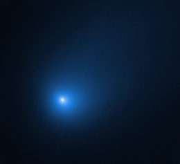
Hubble image of comet 2I/Borisov, captured just after the comet passed perihelion in December 2019. [NASA/ESA/D. Jewitt (UCLA)]
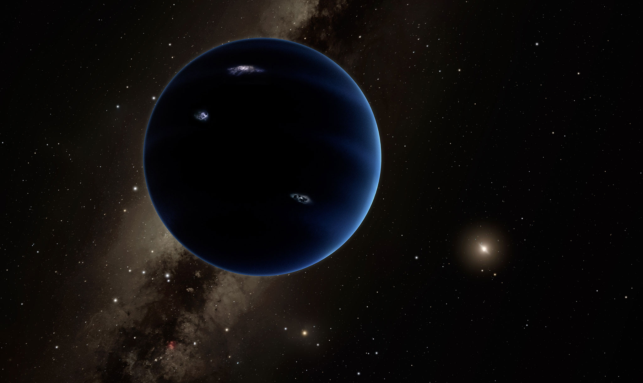
Three and a half years ago, astronomers discovered something in our solar system that had never been seen before: an object from
another star system! Discovered by observatories in Hawaiʻi, this object (illustrated above) was given the name ʻOumuamua, which, in the Hawaiian language, roughly translates to “the first distant messenger.” Two years later, astronomers repeated this feat and discovered yet another
interstellar object (ISO) — this one more cometary in appearance. This object was named after its discoverer,
Borisov. These types of objects were expected to exist but eluded discovery until just now. So where do these objects actually come from? And how often should we expect to find them, now that we know they’re out there? We explore these questions in today’s astrobite.
An Elegant and Simple Model
The authors address these questions by calculating the “differential arrival rate” (Γ) of interstellar objects. Γ is defined as the number of objects that will pass within a given distance of the Sun every year, as a function of their velocity and perihelion (distance of closest approach to the Sun). Γ is the product of three numbers:
- the number density of ISOs (the number of ISOs per unit volume),
- the volume sampling rate of ISOs with a certain velocity and perihelion (the rate that a given volume samples ISOs of a certain type), and
- the probability distribution function of ISO velocities (the probability of an ISO having a particular velocity).
The first order of business is to calculate the number density of ISOs. For this, the authors turn to previous work, where astronomers used the discovery of ʻOumuamua to place a limit on the number of ISOs within a given volume. This estimate uses the detection rate, i.e., how many such objects are detected per year, divided by the amount of volume that the PanSTARRS observatory surveys per year (PanSTARRS was the first survey to detect ʻOumuamua). Even more time has passed since ʻOumuamua was discovered, and since the quality of surveys has improved as well, this work assumes there may be around half as many ISOs per unit volume as previously predicted.
Calculating the volume sampling rate is a bit more complicated, though it is conceptually straightforward. The amount of volume sampled at a given perihelion is just the cross sectional area enclosed by the perihelion multiplied by the velocity of an ISO (area * velocity = volume / time). However, it is imperative to account for “gravitational focusing,” the phenomenon whereby the Sun’s gravity alters the trajectories of smaller bodies passing through the solar system. The basic idea is that objects moving more slowly will be even more likely to be “focused” towards the Sun on their orbit, thus increasing the volume sampling rate for these types of objects. Nonetheless, this calculation only requires the assumption of a typical perihelion.
The last piece of the puzzle is to determine the probability distribution function of ISO velocities. This is the most difficult of the three necessary ingredients to obtain, and for this, we must consult the stars.
Consulting the Stars to Learn about Interstellar Objects
To recap, the authors want to calculate the differential arrival rate, Γ, of ISOs, or how many ISOs arrive in the solar system per unit time. To do this, they need to know their number density, the rate at which a given volume interacts with ISOs with a given velocity, and the probability of finding ISOs with that speed. Above we outlined how the authors determine the first two. However, if we have only ever discovered two ISOs (which are substantially different from each other), how can we possibly determine this last crucial ingredient, the probability distribution function of ISO velocities?
Here the authors make a basic assumption: the velocity distribution of ISOs relative to the solar system is probably similar to the velocity distribution of the host stars from which they originate. It is true that some objects may be kicked from their star systems at extreme velocities, but most are thought to exit with relatively low ejection velocities. This means all we need to do is measure the three-dimensional motion of a representative sample of stars near our solar system. Thankfully, the Gaia spacecraft, launched in 2013, has measured the precise motions of millions of stars, including several hundred thousand near (within 100 pc of) the Sun. After making some quality cuts, the authors use the precise motions of more than 70,000 nearby stars as a proxy for the velocity distribution of ISOs.
The velocity distribution of ISOs encodes the probability of finding an ISO with a particular velocity, since by definition, it describes how many ISOs have certain velocities. The authors combine this information with the two other components needed to calculate the arrival rate Γ of ISOs, and the result is given in Figure 1 below.

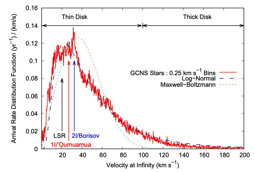
Figure 1: The number of interstellar objects that pass within 1 au of the Sun as a function of their velocity (“at infinity”, prior to entering the solar system). This distribution is Γ, the differential arrival rate. It shows that the majority of ISOs enter the solar system with velocities below 60 km/s. Also highlighted are the velocities of ʻOumumua and Borisov, two different objects discovered that came from beyond the solar system. Unsurprisingly, their velocities are near the median of this distribution. The authors also show the velocity of the local standard of rest (LSR); in this case, the LSR measures the relative velocity of the mean motion of material in the Milky Way at the Sun’s distance from the galactic center compared to the Sun. [Eubanks et al. 2021]
Finally, with the differential arrival rate (Γ) calculated, the authors deduce how many ISOs pass through the solar system with various velocities by integrating Γ across velocities (calculating the area under the red curve in Figure 1). In doing so, the authors predict that on average,
6.9 ISOs pass through the solar system within 1 au of the Sun every year. According to the authors’ estimates,
the vast majority of these objects (92%) will have velocities below 100 km/s. Most objects will have
velocities around 38 km/s, which is the median of the sample. Unsurprisingly, the observed ISO ʻOumuamua has velocities near the peak of this value. Though 2I/Borisov is likely substantially different from ʻOumuamua, it nonetheless shares a similar velocity, suggesting objects like it share similar velocity probability distributions. The authors’ results are neatly summarized in the table below.
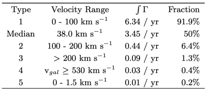
Table 1: According to the type of interstellar object, this table summarizes the velocity range, arrival rate (integral of Γ), and fraction of the total population of detectable ISOs this type of object comprises. These numbers are tabulated for a perihelion of 1 au, meaning these objects would pass relatively close to Earth. Very few fast moving objects are expected to make this journey. [Eubanks et al. 2021]
As an added bonus to this analysis, the authors are able to estimate the probable origins within the galaxy of ISOs with different velocities. It turns out that, depending on where a star is located within the galaxy, it is likely to have a certain velocity relative to the Sun. Stars within the thin disk of the Milky Way move more coherently and are likely to have smaller velocities relative to the Sun (providing Type-1 ISOs, as per the authors’ analysis in the table above); stars within the thick disk have orbits that are more inclined and eccentric, and move even faster (providing Type-2 ISOs); stars within the Milky Way halo, mostly the debris of past accretion events, have even further disturbed and faster orbits relative to the Sun (providing Type-3 ISOs); and the fastest stars are not even bound to our galaxy (providing Type-4 ISOs). Reading off of the table above, we can see that the majority of ISOs will come from the galactic disk. The final group, the slowest moving of them all (Type 5), are objects that appear unbounded but likely originated from the
Oort cloud. These objects, though deemed interstellar due to their unbounded orbits, are simply nudged into the inner solar system through gravitational interactions. With this information, the authors have not only predicted how often we should expect to find ISOs at different velocities, but also where they came from!
There is an incredible amount of science to be excited about when it comes to studying ISOs. These structures not only teach us about other star systems and the Milky Way galaxy, but also teach us about our own solar system by allowing comparison between their compositions and objects found more locally. Especially tantalizing is the prospect of actually rendezvousing with one these objects. Such an endeavor represents what might be our best chance at taking physical samples of material from other star systems on human timescales. With so much on offer, we have reason to suspect such an event may take place in our own lifetimes. One can hope!
Original astrobite edited by Alice Curtin and Ryan Golant.
About the author, Lukas Zalesky:
I am a PhD student at University of Hawaii’s Institute for Astronomy. I am interested in understanding the way galaxies form and evolve over billions of years, as well as gravitational lensing by galaxy clusters. Outside of research I spend my time with animals, exercising, practicing Zen, and exploring the beautiful island of Oahu.


