A Highly Eccentric Journey
Editor’s note: Astrobites is a graduate-student-run organization that digests astrophysical literature for undergraduate students. As part of the partnership between the AAS and astrobites, we occasionally repost astrobites content here at AAS Nova. We hope you enjoy this post from astrobites; the original can be viewed at astrobites.org.
Title: Eccentric Early Migration of Neptune
Authors: David Nesvorný
First Author’s Institution: Southwest Research Institute
Status: Published in ApJL
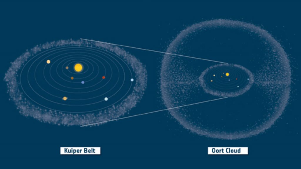
Among the furthest reaches of our solar system, beyond the orbits of the mighty ice giants, lies the Kuiper Belt. This circumstellar disk, roughly twenty times as wide as the asteroid belt, is home to many small bodies (defined by the IAU as any Sun-orbiting body that is neither a planet, dwarf planet, nor satellite), as well as various dwarfs, including what was once the ninth planet. Collectively, these bodies are referred to as Kuiper Belt Objects (KBOs), which are themselves a subset of Trans-Neptunian Objects (TNOs). Understanding the collective orbits of KBOs provides important insights into the evolutionary history of our early solar system.
Neptune, like other outer gas giants, is known to have migrated in the past and interacted with KBOs. We can predict what Neptune’s migratory orbit was like by simulating different planetary migration scenarios for the outer planets, seeing how they affect KBOs, then finding the parameters that best match currently observed KBO orbits. Today’s paper examines a group of KBOs within a specific range of orbital parameters whose current orbits are unable to be accounted for in simulations if Neptune migrated with a low orbital eccentricity (e << 0.03). Instead, better results are obtained if Neptune migrated with a higher eccentricity of e ~ 0.1.
Space For The Travelling Planet
Under the current framework for accounting for the dynamical evolution of the early solar system, Neptune is known to have migrated into a higher orbit, subsequently interacting with the Kuiper Belt and its various KBOs. After this migration, Neptune’s orbit slowly decayed and circularised, causing the planet to move inward to its current position today. This migration is noted to have altered the distribution of inclinations and eccentricities of KBOs, and (in conjunction with other migrations by Uranus, Saturn, and Jupiter) is theorised to be responsible for scattering many KBOs and other planetesimals into the inner solar system (the Late Heavy Bombardment). Studies focusing on this period of instability have aimed to constrain the eccentricity of Neptune’s migration. There are many factors to consider, such as tidal interactions and possible orbital resonances with KBOs or the other gas giants, dynamical friction, and Kozai cycles (which cause eccentricity and inclination to oscillate).
This study definitively rules out the low-eccentricity migration scenario, and instead provides support to an excitation scenario wherein Neptune had an eccentricity of e ~ 0.1. The data used to fine-tune the simulations was obtained from the Outer Solar Systems Origin Survey (OSSOS), which identified a population of KBOs with semimajor axes between 50 and 60 AU, a perihelion distance greater than 35 AU, and an inclination of less than 10 degrees. Figure 1 shows all KBOs with semimajor axes between 50 and 60 AU plotted by eccentricity, with the OSSOS samples highlighted as blue triangles. Simulations show that the existence of this population is easily accounted for in the high-eccentricity model; here bodies originally at around 30 AU are scattered into higher orbits (50 to 60 AU), where they subsequently interact with Neptune due to mean motion resonances. The bodies eventually decouple, forming the specific 50–60 AU population that we see today.
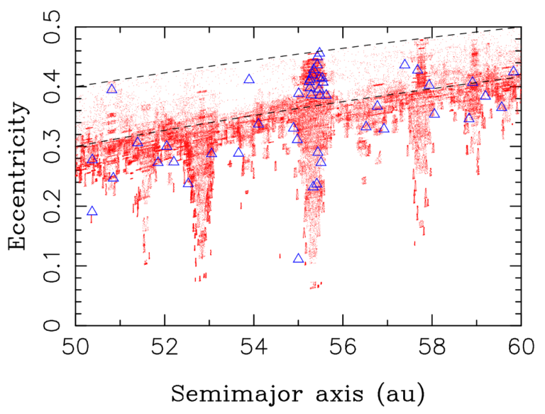
Figure 1: A plot of modelled orbits of KBOs with semimajor axes between 50 and 60 AU plotted by eccentricity (shown as red dots), with the OSSOS detections overlaid as blue triangles. [Nesvorný 2021]
A Wandering Neptune
Importantly, this study provides a key physical explanation as to why the low-eccentricity model cannot work in practice. Were Neptune to have a low eccentricity, the mean motion resonances would not be as effective, and so the scattered KBOs would need to decouple via Kozai resonances. However, in Kozai cycles, as eccentricity decreases, inclination must increase. The KBOs in this situation would thus be unable to satisfy the target parameter range of having less than 10 degree inclination (see Figure 2, which shows this exclusionary zone). The only other explanation for their existence is that these KBOs originated in situ, in some hypothetical disc that was perturbed by other means.
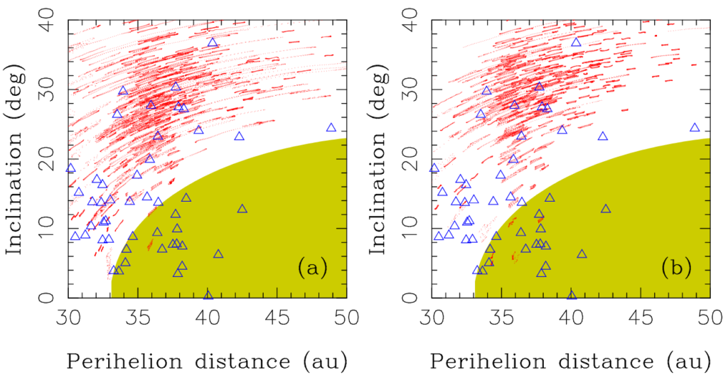
Figure 2: Orbital inclinations and perihelia for KBOs with semimajor axes between 50 and 60 AU. Left and right panels correspond to two different dynamical models. Blue triangles denote the OSSOS samples. The olive shaded region is the excluded region in which objects scattered by a low-eccentricity Neptune cannot exist. The fact that OSSOS samples do exist rules out the low-eccentricity case. [Nesvorný 2021]
And Yet They Moved
The Kuiper Belt remains an active frontier for research into the dynamical evolution of the early solar system. Not only does accounting for the orbital properties of KBOs yield insights into the evolutionary history of the outer planets, but it enhances our understanding of the physical processes at play — from mean motion resonances to Kozai cycles — allowing us to better constrain the orbital parameters of migrating planets. This is important given the rise of exoplanetary science, and the need to account for the many exotic planetary configurations that have been discovered. Only then can we build a complete picture of how planetary migration affects planetary systems.
Original astrobite edited by Gloria Fonseca Alvarez.
The author would like to acknowledge the Whadjuk peoples of the Noongar nation, the traditional custodians of the land on which this post was written, and pays respects to Elders past and present.
About the author, Mitchell Cavanagh:
Mitchell is a PhD student in astrophysics at the University of Western Australia. His research is focused on the applications of machine learning to the study of galaxy formation and evolution. Outside of research, he is an avid bookworm and enjoys gaming, languages and code jams.