Rogue Exomoons
Editor’s note: Astrobites is a graduate-student-run organization that digests astrophysical literature for undergraduate students. As part of the partnership between the AAS and astrobites, we occasionally repost astrobites content here at AAS Nova. We hope you enjoy this post from astrobites; the original can be viewed at astrobites.org.
Title: On the Detection of Exomoons Transiting Isolated Planetary-Mass Objects
Authors: Mary Anne Limbach et al.
First Author’s Institution: Texas A&M University
Status: Published in ApJ
When faced with the sheer beauty of shimmering stars emblazoned across a night’s sky, it’s hard not to imagine that there are innumerable other worlds out there — entire planets teeming with alien life, or ruins of once-great civilisations. Until recent decades, such imagination was confined to the realm of science fiction, but in 1992 came the first detection of an exoplanet: a planet outside our solar system.
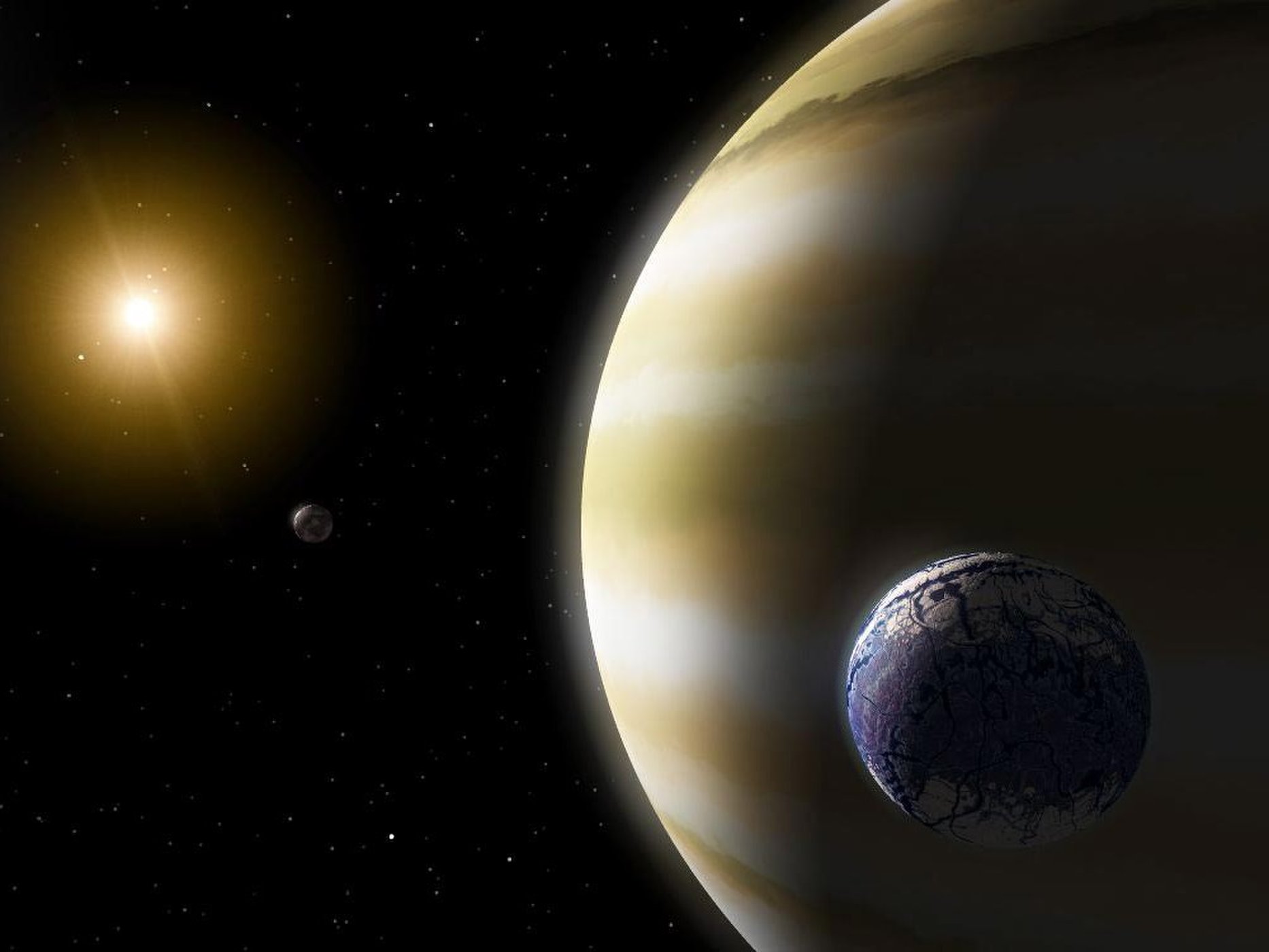
Artist’s depiction of an Earth-like exomoon orbiting a gas-giant planet. [NASA/JPL-Caltech]
Sunless Skies
Rogue planets are not bound to a planetary system. Instead, they roam free throughout the galaxy, bathed in darkness and lit by no sun. This makes it much easier to detect exomoons that orbit IPMOs compared to those orbiting ordinary exoplanets. The authors estimate that for over half of all known IPMOs, the sensitivity of the upcoming James Webb Space Telescope (JWST) is enough to detect the presence of an exomoon with similar characteristics to Jupiter’s moon Ganymede. Before planning an exomoon hunt, one must first consider observational constraints. One of the most important is the probability of observing a transit in the first place. Simulations have demonstrated that the formation of moons is common — with at least one large moon forming in roughly 80% of planetary systems — and that these moons often resemble the Galilean moons with respect to their sizes and orbital configurations.
Moonlight Sonata
It is therefore sensible to model probabilities based on moons in our own solar system, such as those orbiting the gas giants. The authors first model the transit probabilities for the solar system gas giant moons — that is, they find the probabilities that a moon will cross the face of the gas giant — with respect to some randomly oriented observer located outside the solar system.
Figure 1 shows the probabilities of observing at least one transit in some system of planets, as well as the observed transit depths. In this case, the transit depth refers to the fractional dip in the light curve of a planet as it is transited by its moon. Supposing that we observed 10 planets with moons, the probability of observing a transit of an Io-like moon is about 85%. For a Europa-like moon, the transit probability drops to 70%, while transits of Mercury-like and Jupiter-like moons are much rarer, at 10% and less than 1% probability respectively.
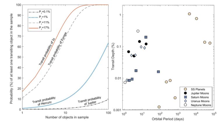
Figure 1: Left: Probability of observing at least one transit as a function of the number of objects (exoplanets) in the sample. The curves represent different solar system objects. Right: Percentage transit depth as a function of orbital period for various planets and moons in our solar system. [Limbach et al. 2021]
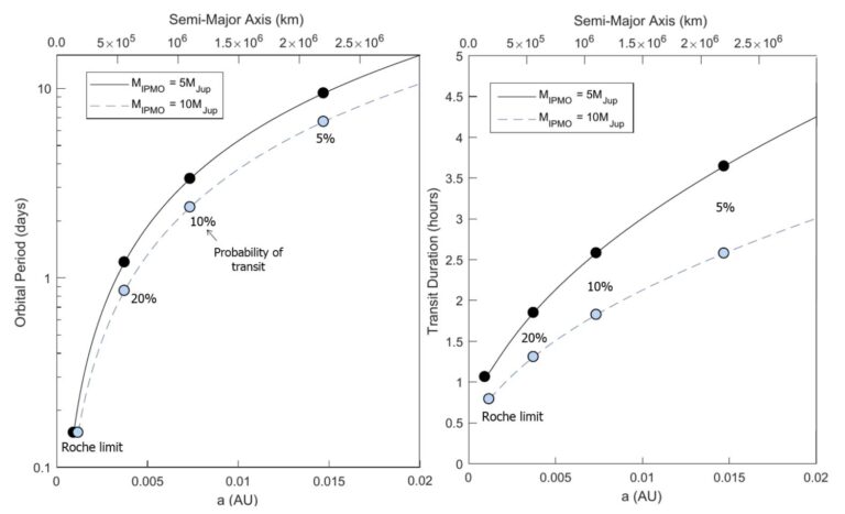
Figure 2: Left: Orbital period of an exomoon versus its orbital distance (in both astronomical units and kilometres). The curves denote super-Jupiter mass IPMOs with transit probabilities listed. The Roche limit is the closest the moon can orbit the planet. Right: Similar to the left panel, but with transit duration on the vertical axis. [Limbach et al. 2021]
Roguelike Exomoons
The main advantage of looking for moons around IPMOs is that high-contrast and high-resolution imaging is not needed; there is no interference from a nearby host star to drown out any signal. Instead, current ground telescopes can observe IPMOs with very high precision. Next-generation space-based telescopes, such as the imminent JWST, will further improve this precision by an order of magnitude.
Figure 3 shows the radius of moons orbiting Jupiter-mass exoplanets versus the photometric precision required to accurately detect their transit. Current high-contrast imaging of stellar-bound exoplanets can only detect moons at least as big as Neptune. With IPMOs, ground-based imaging allows for the detection of Earth-sized moons. With the JWST, it will be possible to detect Ganymede-sized moons, and even moons down to the size of Titan or Io! The authors calculate that the JWST will be able to detect Ganymede-sized moons around over half of all known IPMOs.
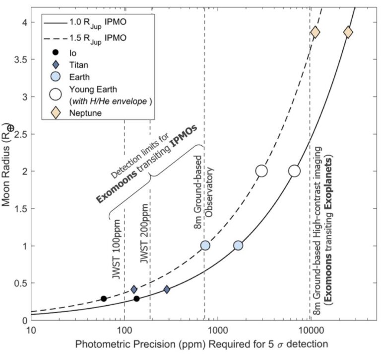
Figure 3: Exomoon radius (in units of Earth radii) versus the photometric precision required for an accurate transit detection (logarithmic scale). Smaller precision values correspond to higher resolutions. The solid and dotted curves denote Jupiter mass and 1.5 x Jupiter mass IMPOs, with the shapes corresponding to the sizes of orbiting moons. Vertical lines denote the sensitivity limits of current/future observations. [Adapted from Limbach et al. 2021]
Sic Mundus Creatus Est
Exomoons are believed to be just as common as exoplanets, with at least one large moon forming around approximately 80% of simulated planets. Rogue exoplanets can be observed with a higher photometric precision since there is no glare/interference from a nearby host star. Moon–planet transits are also relatively common, and more than half of all known IPMOs are bright enough to allow for the detection of a Ganymede-sized moon. However, the authors propose a minimum observing time of 50 hours, which adds up to nearly 17 weeks of combined observing time for the 57 known IPMOs. The authors note that IPMO exomoons are among the most accessible candidates for detecting habitable worlds (in this case, the moon is warmed by tidal heating rather than by a star). Potentially habitable IPMO exomoons would not only lend insight into the processes governing planet formation, but could also offer a window into the conditions of the primordial Earth, thus allowing us to place a timescale on the development of life itself.
Original astrobite edited by Ryan Golant.
About the author, Mitchell Kavanagh:
Mitchell is a PhD student in astrophysics at the University of Western Australia. His research is focused on the applications of machine learning to the study of galaxy formation and evolution. Outside of research, he is an avid bookworm and enjoys gaming, languages and code jams.


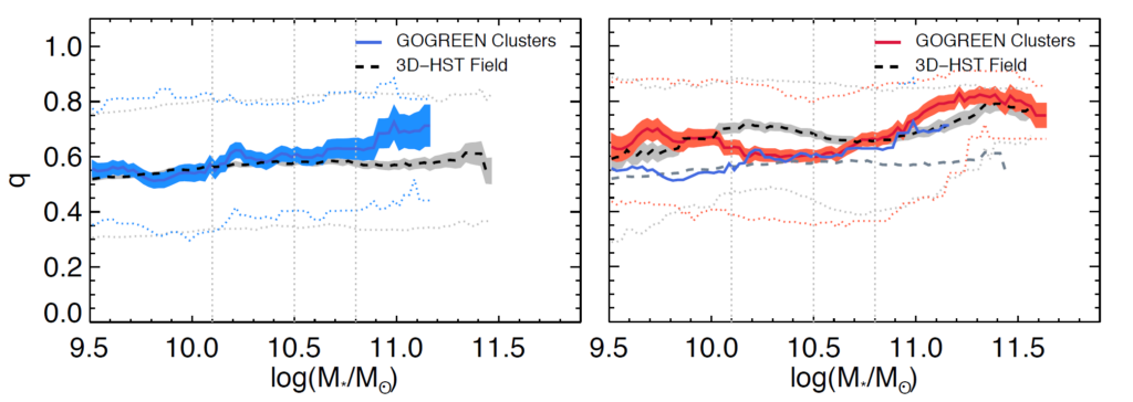
 Galaxies in Distant Clusters")