
How a Moon-Sized Deep Impact Affected Early Life on Earth
Editor’s Note: Astrobites is a graduate-student-run organization that digests astrophysical literature for undergraduate students. As part of the partnership between the AAS and astrobites, we occasionally repost astrobites content here at AAS Nova. We hope you enjoy this post from astrobites; the original can be viewed at astrobites.org.
Title: Large Impacts onto the Early Earth: Planetary Sterilization and Iron Delivery
Authors: Robert I. Citron and Sarah T. Stewart
First Author’s Institution: University of California, Davis
Status: Published in PSJ
The early Earth wasn’t your typical summer break vacation destination. During the Hadean Eon (4.5–4.0 billion years ago), Earth was an extremely hostile environment and was frequently bombarded by asteroids. Yet, somehow, life on Earth could have emerged during this time.
This story begins with a noteworthy event during the Hadean Eon: a now long-gone Mars-sized planet called Theia slammed into Earth. The massive impact blew off a large amount of debris that started to circle the new Earth–Theia merger and eventually formed the Moon. This proposed sequence of events is known as the Giant Impact Hypothesis. Theia’s impact melted Earth’s entire crust several kilometers deep, creating an environment not very favorable for any form of life that we know of and very likely sterilizing anything already present on Earth. After all the turmoil of the impact settled down, life on Earth (in principle) could have formed shortly after, a mere 4.5 billion years ago. Reality, as it turns out, may have run less smoothly.
As a deeply studied subject, the origin of life has been described by several proposed hypotheses. A popular hypothesis states that it all began with the formation of amino acids and RNA molecules. Because our present-day atmosphere and oceans are oxidizing (noticed iron rusting? Maybe some fire?), spontaneously forming these molecules is difficult. But what about all those lifeforms we see today? They needed to come from somewhere. Well, to actually form these amino acids and RNA molecules on a global scale, we would need a reducing atmosphere or ocean. And how better to create one than slamming a huge rock full of reducing material (like iron) into Earth?
Reducing an Atmosphere 101
After the Theia impact, but still during the Hadean Eon, Earth endured a large amount of impacting asteroids of varying sizes, which were sling-shotted to the inner solar system by Jupiter and Saturn. The authors of today’s article wanted to know which objects under which conditions can actually create a (temporarily) reducing atmosphere or ocean on Earth, ultimately opening the way to forming the building blocks of life. Instead of really slamming various rocks on Earth, the authors ran smoothed particle hydrodynamics (SPH) simulations of large objects (the projectiles) colliding with an Earth-like planet (ominously called the target). To account for several possible scenarios, illustrated in Figure 1, the authors varied the impacting object’s mass, velocity, and the angle at which it strikes Earth.
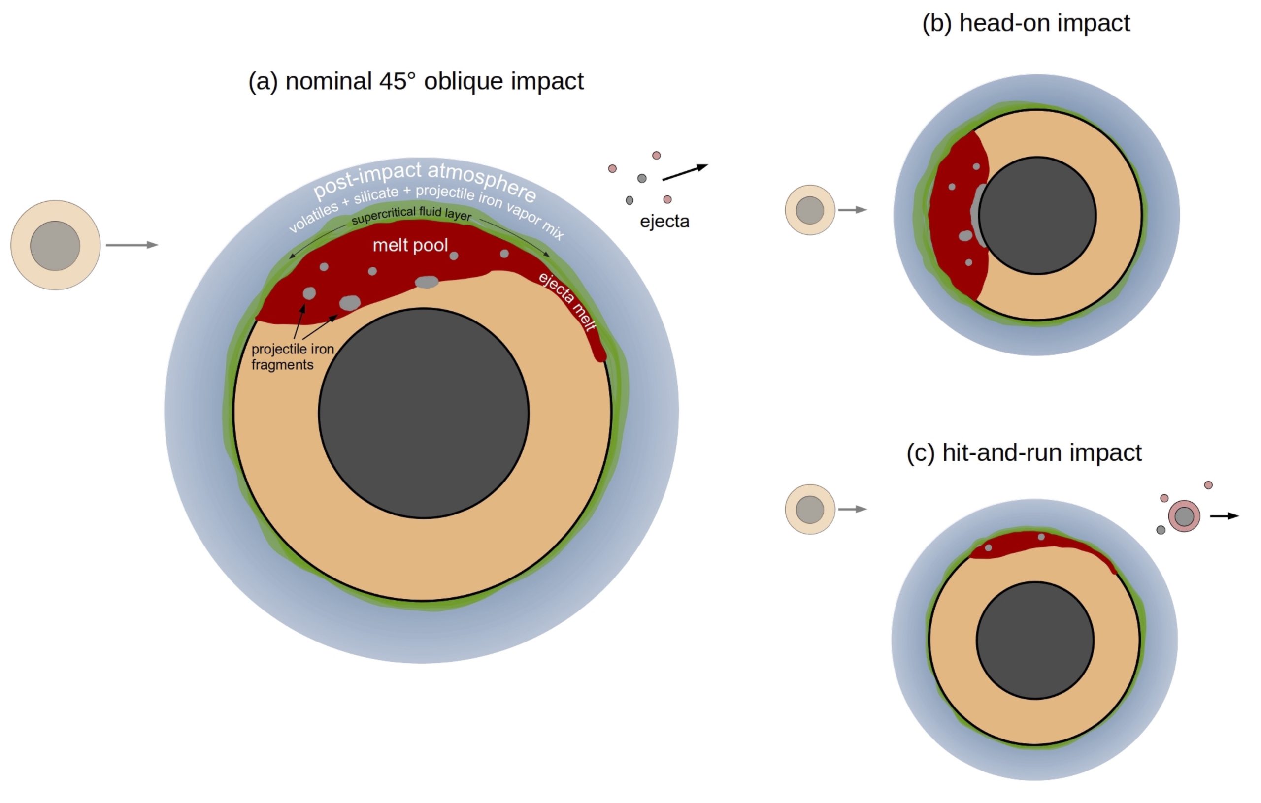
Figure 1: Effect of different impact angles of a large object colliding with Earth, with the distinction between the atmosphere (blue), the mantle (orange), and the core (dark gray). Different angles lead to different degrees of surface melting (red). [Citron & Stewart 2022]
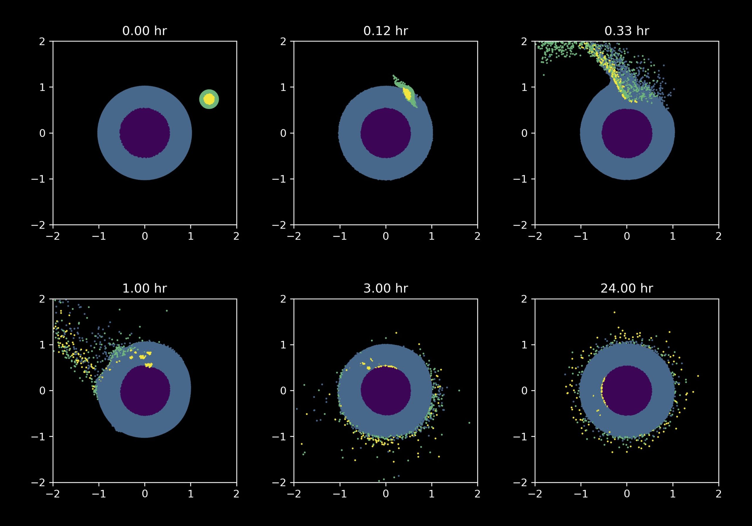
Figure 2: Simulation of a smaller object colliding with Earth. Here, the object mass is 25% of the Moon’s mass, the impact velocity is 1.5 times Earth’s escape velocity, and the impact angle is 45°. The mantle and core materials of Earth and the impacting object are color-coded to see where they eventually land, if at all. This simulation shows that the object is shattered on Earth’s surface; the colliding object’s mantle material — forsterite — is mainly scattered around Earth or resides on its surface, while the heavier core material from the object — iron — mainly sinks in large chunks to Earth’s interior. Part of the iron from the object, however, remains scattered in the atmosphere, where it will act as a reducing agent. The spatial dimensions are expressed in Earth radii. [Citron & Stewart 2022]
However, this study has shown that it takes a larger object than previously estimated to fully sterilize the early Earth’s exterior by melting its whole surface; such an object would need to have more than 25% of the Moon’s mass. As objects this size were rare even during the Hadean Eon, the chances of a mass extinction by space rocks are lower than previously expected. Even the ocean-evaporating asteroids do not necessarily sterilize Earth if early life occurred under the planet’s surface. Moreover, remember the Moon-sized asteroids needed to fully reduce the atmosphere and oceans? Turns out we don’t need that kind of overkill (pun intended). Multiple smaller objects slamming into Earth could reduce the atmosphere or ocean enough to create favorable conditions for spontaneous RNA formation.
In any case, if life emerged from a post-impact world, it would be due to the right asteroids at the right time. Too small, and the kick-starter for life wouldn’t occur. Too large, and any progress made so far would be wiped out. Considering the fact that you are reading this post, it seems our very, very far forebears weren’t out of luck!
Original astrobite edited by Sarah Bodansky.
About the author, Roel Lefever:
Roel is a first-year astrophysics PhD student at Heidelberg University. He works on massive stars and simulates their atmospheres and outflows. In his spare time, he likes to hike and bike in nature, play (a whole lot of) video games, play and listen to music (movie soundtracks!), and read (currently The Wheel of Time, but any fantasy really).


