Young, Cool, and on Edge: An Unstable Protoplanetary Disk
Editor’s Note: Astrobites is a graduate-student-run organization that digests astrophysical literature for undergraduate students. As part of the partnership between the AAS and astrobites, we occasionally repost astrobites content here at AAS Nova. We hope you enjoy this post from astrobites; the original can be viewed at astrobites.org.
Title: Formation of Dust Clumps with Sub-Jupiter Mass and Cold Shadowed Region in Gravitationally Unstable Disk around Class 0/I Protostar in L1527 IRS
Authors: Satoshi Ohashi et al.
First Author’s Institution: RIKEN Cluster for Pioneering Research, Japan
Status: Published in ApJ
When a cloud of gas in space has enough mass, the gravitational forces from all the gas overwhelm the gas pressure keeping the cloud puffed up, and the cloud collapses under its own gravity to form a star. If the cloud is initially rotating, the contraction of the gas will magnify that rotation due to the conservation of angular momentum — imagine spinning on a desk chair and pulling your legs in towards your body. The rotation also drives material towards the equatorial plane, ultimately resulting in a so-called protoplanetary disk — a flattened disk of leftover gas and dust orbiting the newly formed star.
The protoplanetary disk that birthed the planets in our solar system is long gone, so we need to look to stars much younger than our Sun to study these planetary nurseries. Today’s authors present a detailed analysis of a particular protoplanetary disk — one that is gravitationally unstable.
Remember the gravitational instability that formed the star from a cloud? Well, the disk can be unstable to its own gravity, too, when the pressure and rotational forces are too small to prevent collapse. This can occur if the disk is very massive and also very cool. Gravitational instability in disks is one possible way of manufacturing giant planets. It causes the disk to fragment into many small blobs of gas, which then collapse into planets. Thus, understanding how gravitational instability begins is an important piece of the puzzle in understanding the formation of the diverse range of planetary systems discovered over the last 20 years.
Observing an Edge-On Protoplanetary Disk
Two excellent tools for observing protoplanetary disks are the Atacama Large Millimeter/submillimeter Array (ALMA) and the Jansky Very Large Array (JVLA). Both use an array of radio dishes that look at the target in unison, acting as one massive telescope. Both can observe at different wavelengths, called bands, which can be combined to produce a more complete picture of the disk.
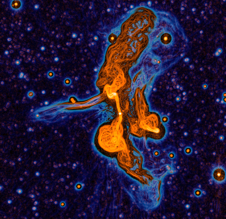
The disk observed by today’s authors is around the very young (less than 100,000 years) star Lynds 1527 (L1527) IRS in the Taurus molecular cloud at a distance of 447 light-years. The disk is viewed nearly edge on, its host star is still accreting, and the disk has not yet fully formed. Each band penetrates the disk to a different depth, so the observation will look very different depending on the filter. Figure 1 shows three ALMA images (bands 3, 4, and 7) and one JVLA image (Q band).
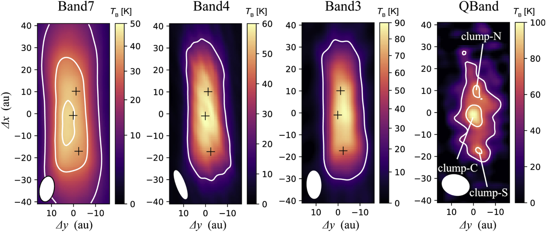
Figure 1: ALMA images (Band 7, 4, and 3) and JVLA image (Q band) of the L1527 protoplanetary disk viewed edge on. The clumps detected in the Q band are marked with black crosses in the other panels. The white ellipse in the bottom left of each panel indicates the image resolution. [Ohashi et al. 2022]
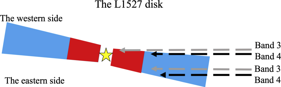
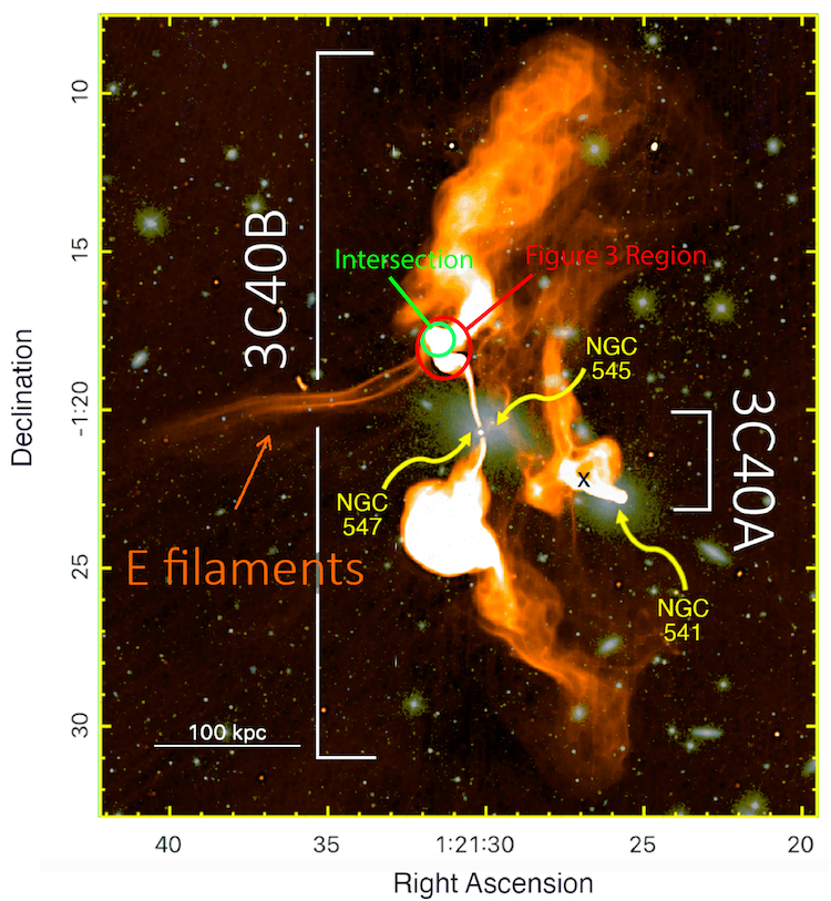
Figure 2: Sketch of L1527’s disk as viewed from Earth. The hot regions (red) on the near side are obscured by the flared outer disk (blue), so the near side appears slightly hotter in temperature maps. [Ohashi et al. 2022]
Assessing Gravitational Instability
A gravitationally unstable disk is characterized by a distinctive spiral structure. The problem is we can only view this disk edge on, so we can’t see the spiral structure — much like how the Milky Way’s spiral structure isn’t visible from Earth.
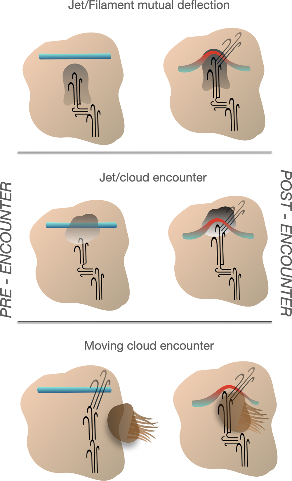
The authors resolved this issue by assessing the stability of the L1527 disk using Toomre’s stability analysis with measured values for temperature and surface density. They find that the disk is expected to be gravitationally unstable. The left panel of Figure 3 shows the spiral structure typical of a gravitationally unstable disk in the face-on view. If we were to look at this model disk from an edge-on, 90°-rotated view, we’d see two high-density regions flanking the center of the disk (right panel of Figure 3). This almost reproduces the shape of the Q-band observation (rightmost panel, Figure 1), so the authors conclude that L1527’s disk is indeed likely to be gravitationally unstable.
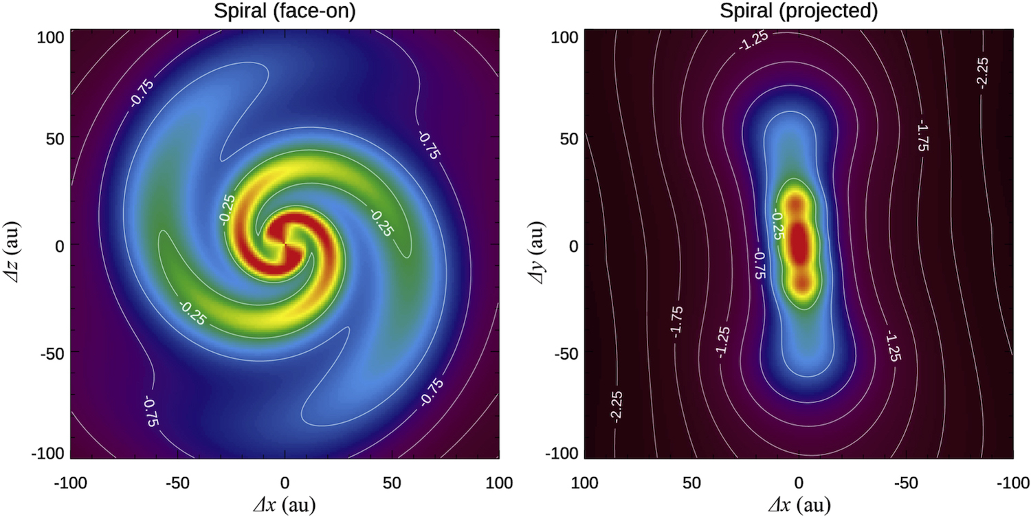
Figure 3: Model of a gravitationally unstable disk. If a massive disk cools enough such that its gas pressure cannot withstand the gas’s self-gravity, it starts to fragment and form a spiral structure (left panel, face-on view). The spiral structure projects two clumps on the edge-on view (right panel). [Ohashi et al. 2022]
Original astrobite edited by Sasha Warren.
About the author, Konstantin Gerbig:
I’m a PhD student in Astronomy at Yale University. I’m interested in the theory of (exo)planets and protoplanetary disks and do hydro simulations thereof. I also like music, as well as dancing salsa and tango.