How To Jump-Start a Supermassive Black Hole
Editor’s note: Astrobites is a graduate-student-run organization that digests astrophysical literature for undergraduate students. As part of the partnership between the AAS and astrobites, we occasionally repost astrobites content here at AAS Nova. We hope you enjoy this post from astrobites; the original can be viewed at astrobites.org.
Title: Exploring the AGN–Ram Pressure Stripping Connection in Local Clusters
Authors: Giorgia Peluso et al.
First Author’s Institution: INAF-Padova Astronomical Observatory, Padova, Italy
Status: Published in ApJ
Current theories suggest that most galaxies — if not all — contain a supermassive black hole in their centre, with masses anywhere from millions to billions of times that of our Sun. This theory was bolstered in 2019, when the Event Horizon Telescope took the first ever photograph of a black hole in the centre of the nearby elliptical galaxy M87, and in 2020, when Reinhard Genzel and Andrea Ghez were awarded the Nobel Prize in Physics for discovering a supermassive black hole at the centre of our own galaxy.
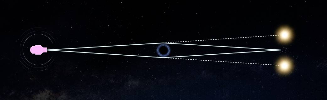
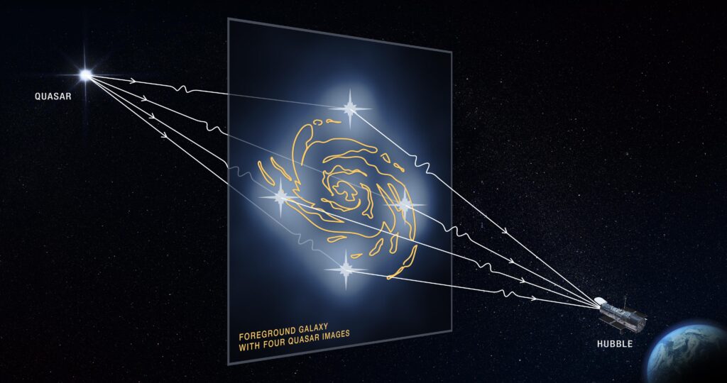
With their enormous density and gravitational fields, black holes are some of the most extreme objects in the universe. Consequently, material that is pulled towards a supermassive black hole can be accelerated almost to the speed of light. If enough material is present, it can form an accretion disk — an incredibly hot structure that feeds material into a black hole and converts this mass into energy, which is emitted as light. A supermassive black hole surrounded by an accretion disk is known as an active galactic nucleus (AGN) as shown by the artist’s impression in Figure 1.
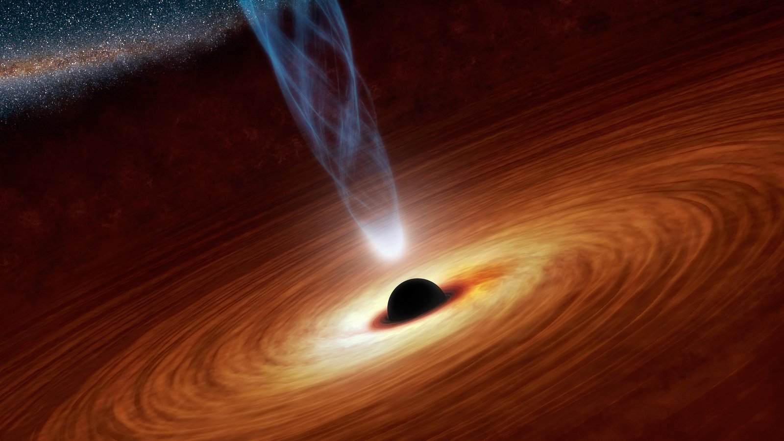
Figure 1: Artist’s impression of an AGN, with a central black hole surrounded by a flat, rotating accretion disk. Some AGNs emit narrow, powerful jets of material — this can be seen above the black hole. [NASA/JPL-Caltech]
It’s Tough to Stay Cool Under Pressure
Galaxy clusters are huge objects containing up to several thousand galaxies. Between these is a sea of hot gas called the intracluster medium. As galaxies sail through this ocean, drag forces from the intracluster medium can cause gas in the galaxies to be stripped away, leading to tails of gas streaming out in their wake. This process is known as ram-pressure stripping. In this article, the authors investigate whether these stripped galaxies are more likely to have an AGN in their centres.
To do this, they use observations of 115 galaxies that are currently undergoing ram-pressure stripping within clusters, taken from multiple different astronomical surveys. These galaxies are compared to a control sample of 782 star-forming galaxies taken from field regions (i.e., not in clusters) of the MaNGA survey. These galaxies are then tested to see whether they contain AGNs by looking at their emission of light at different wavelengths and placing them on a BPT diagram (a commonly used method for identifying AGNs).
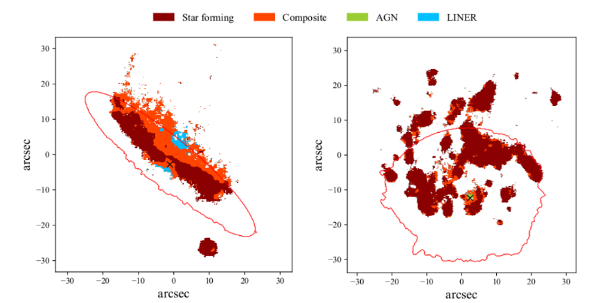
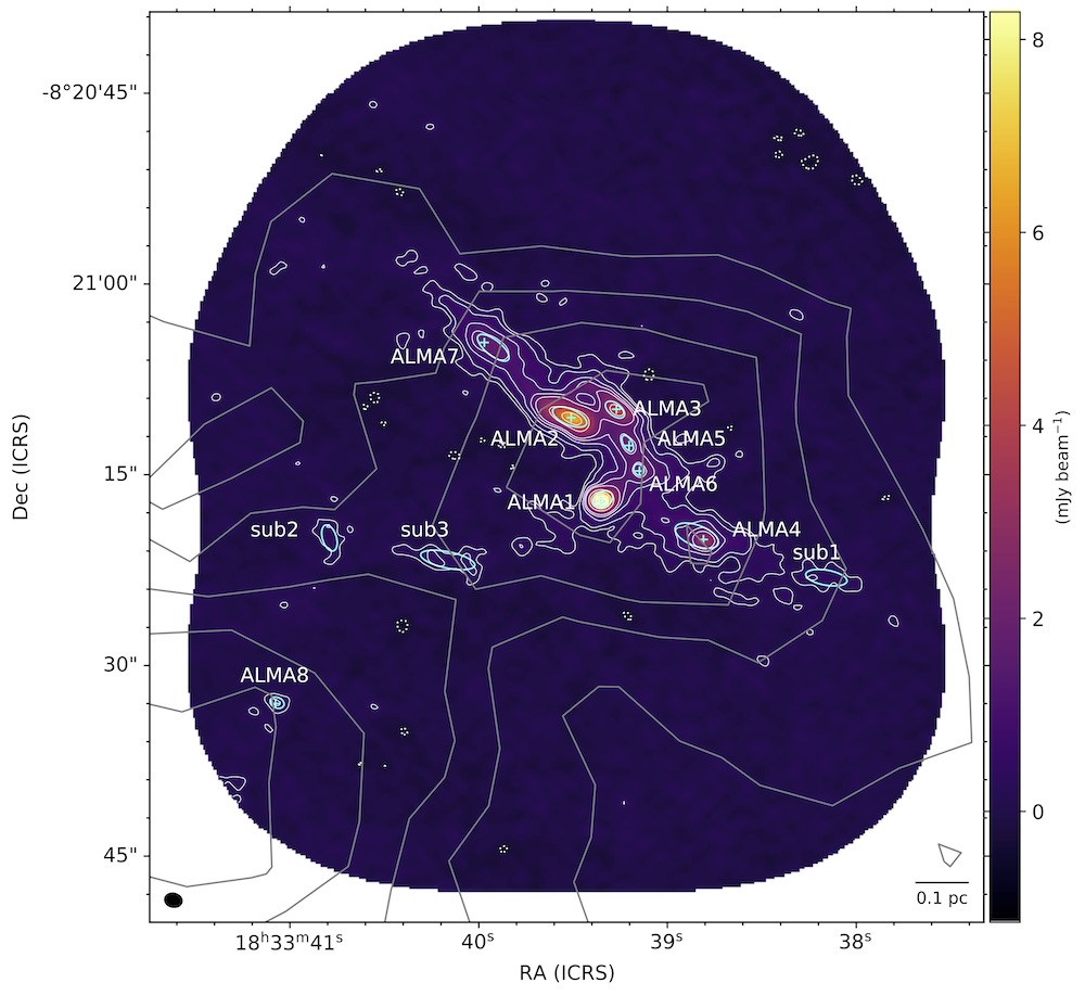
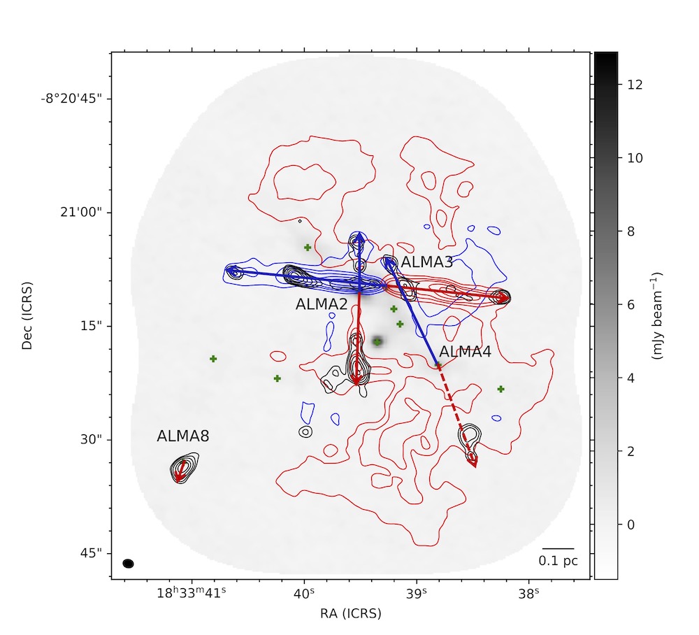
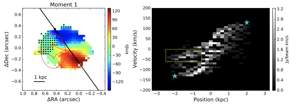
Figure 2: Examples of two ram-pressure stripped galaxies from today’s paper. The gas in these galaxies is shown in red and orange, and the AGN regions are shown in green and blue — some AGN are identified indirectly by LINER emission. The red contours show the edge of the galactic disks, demonstrating how the gas has been stripped away and is trailing behind the galaxies. [Adapted from Peluso et al. 2022]
Fire Up the AG-Engines!
These results are exciting, and tell us that there is a close connection between AGNs and ram-pressure stripping. One potential explanation comes from the fact that the intracluster medium, which causes the stripping of a galaxy’s gas, can also increase the external pressure on a galaxy. This pressure can compress the gas in the galaxy, triggering star formation and causing gas to spiral inwards towards the galaxy centre, resulting in the formation of a luminous accretion disk. Furthermore, triggering an AGN can result in gas being thrown out of a galaxy, leading to the tails of jettisoned gas that are attributed to ram-pressure stripping.
There are several caveats in this article. For example, this work only compares field galaxies to a very specific type of cluster galaxies — those with clear signs of ram-pressure stripping. The authors explain that future studies involving larger numbers of galaxies will be able to constrain their results even further.
Since one third of the non-stripped galaxies also contain AGNs, ram-pressure stripping clearly isn’t the only possible cause of AGN ignition. However, the impact of ram-pressure stripping shown in this article is a valuable clue that will help us move towards a better understanding of what causes these huge cosmic light bulbs to switch on.
Original astrobite edited by Lili Alderson.
About the author, Roan Haggar:
I’m a PhD student at the University of Nottingham, working with hydrodynamical simulations of galaxy clusters to study the evolution of infalling galaxies. I also co-manage a portable planetarium that we take round to schools in the local area. My more terrestrial hobbies include rock climbing and going to music venues that I’ve not been to before.