
Counting Clusters to Probe Ancient Star Formation
Editor’s note: Astrobites is a graduate-student-run organization that digests astrophysical literature for undergraduate students. As part of the partnership between the AAS and astrobites, we occasionally repost astrobites content here at AAS Nova. We hope you enjoy this post from astrobites; the original can be viewed at astrobites.org.
Title: NGC5846-UDG1: A Galaxy Formed Mostly by Star Formation in Massive, Extremely Dense Clumps of Gas
Authors: Shany Danieli et al.
First Author’s Institution: Princeton University
Status: Published in ApJL
Stars can find a home in many different places: some reside in galaxies, whereas others can reside in tightly bound star clusters, which themselves orbit galaxies. The stars that exist in the densest, oldest star clusters — globular clusters — formed in extreme conditions at very early times in regions of space with extremely high gas pressures. Globular clusters are ancient relics encoding information on conditions for star formation in the early universe.
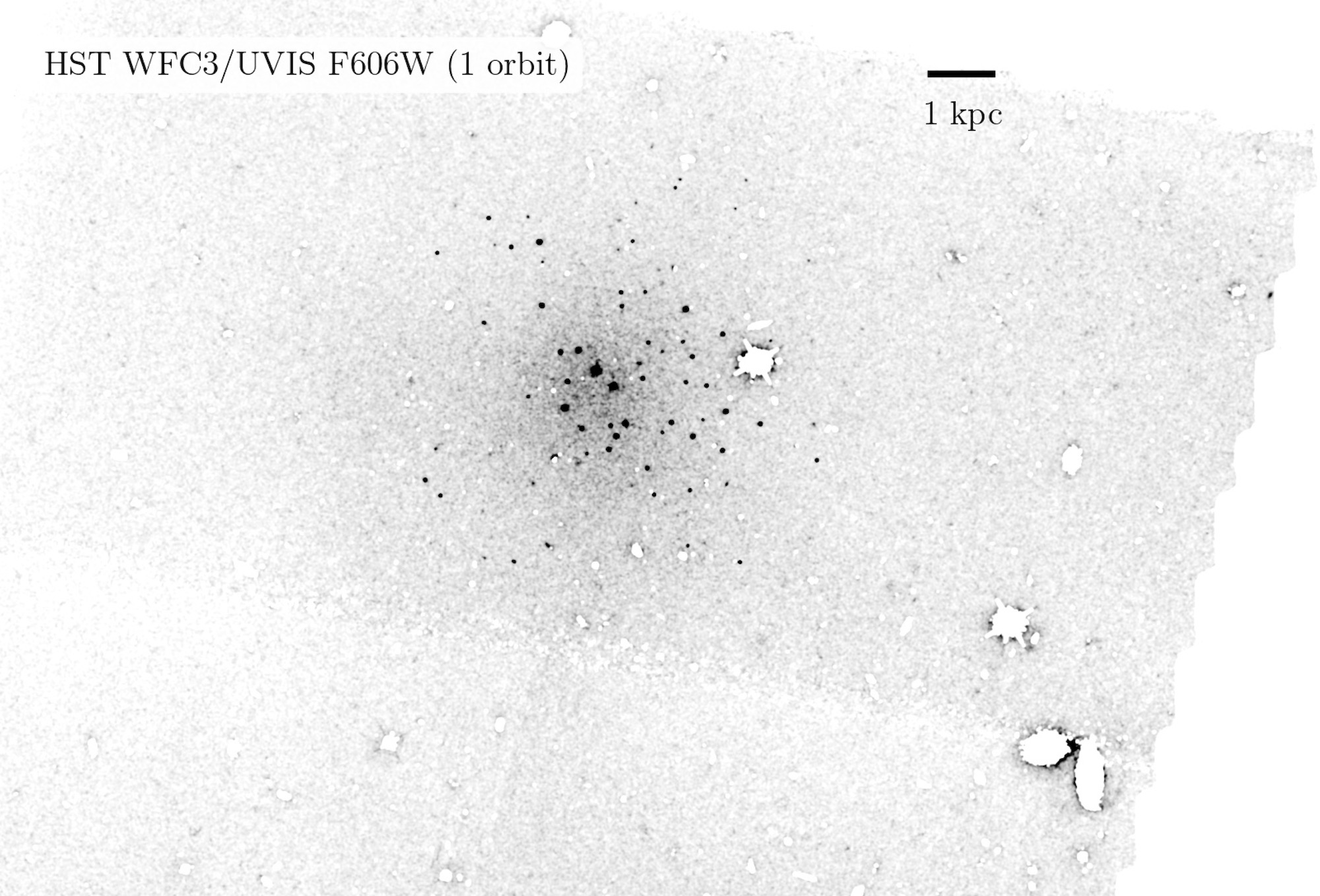
Figure 1: V-band image of UDG1 (diffuse grey points) and its globular cluster candidates (black points). [Adapted from Danieli et al. 2022]
A Galaxy Rich in Globular Clusters
A key result of today’s article is that UDG1 has a significantly higher number of globular clusters than would be expected for a galaxy of its mass, with the tally coming in at 54 (+/- 9)! In addition to the number of globular clusters, the authors also estimate the total light from the clusters relative to the total light in the galaxy itself. The authors find that the globular clusters currently emit 13% of the total light of the galaxy, meaning that 13% of this galaxy’s stars reside in globular clusters — this is the highest fraction of stars in globular clusters known for any galaxy to date, and it’s 100 times larger than the globular cluster fraction of the Milky Way!
While the current proportion of stars in globular clusters for UDG1 is 13%, this figure was likely much higher at earlier times due to the dynamical evolution of these clusters. Globular clusters are expected to interact with their environment and lose mass (or be completely destroyed) via tidal stripping over time. The stars that are lost from the clusters may end up contributing significantly to the stellar content of the galaxy itself (see this astrobite for more).
These mass-loss processes can lead to globular cluster systems losing up to 80–90% of their stellar mass content over their lifetime. The authors use an analytical model to estimate the original cluster fraction (before any mass loss processes occurred) from the current cluster fraction of 13%. They find that the original cluster fraction is likely to have been 65%, indicating that the majority of the stars in this galaxy at present day originally formed in bound clusters from extremely dense gas clumps.
These results are summarised in Figure 2, which displays the cumulative proportion of mass in globular clusters (currently observed clusters in black; the initial cluster model in purple (before mass loss effects); and Milky Way values in orange).
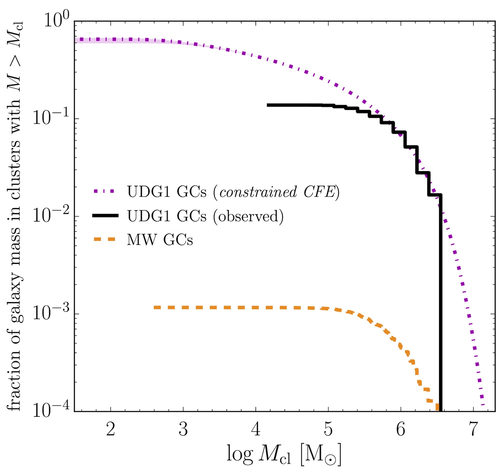
Figure 2: The cumulative fraction of galaxy mass in globular clusters for NGC5846-UDG1 in comparison to the Milky Way. The black line shows the current observed values, the purple dotted line shows the modelled values expected at the time of formation, and the orange dashed line shows the current Milky Way values. Mcl refers to the total stellar mass of the globular clusters. [Adapted from Danieli et al. 2022]
Implications for Star Formation
The large difference between the Milky Way and UDG1 globular cluster fractions highlights the rare conditions under which UDG1 originally formed. Globular cluster formation (and subsequent destruction) is very likely to have been the dominant star formation mode for UDG1, with these stars originally forming from extremely dense, high-pressure gas clumps. This idea is supported by the fact that the spatial distribution and ages of the cluster stars versus the galaxy stars in UDG1 are very similar, indicating that the galaxy’s stars likely originated from disrupted globular clusters.
It is unlikely that UDG1 is the only galaxy of its kind. The authors note that there are hints that some ultra-diffuse galaxies in the Coma cluster have similarly high globular cluster fractions. The uncertainties on these measurements are high since the galaxies in the Coma cluster are located farther away, but it’s still a promising indicator that star formation through extremely dense clumps at early times may be a viable way to build a galaxy!
Original astrobite edited by Gloria Fonesca Alvarez.
About the author, Katy Proctor:
I am a first-year PhD student at the International Centre for Radio Astronomy Research at the University of Western Australia. My research is focused on using cosmological simulations to study the build up of stellar halos. Outside of research, I can usually be found climbing up walls or playing guitar.


