Astrobites RSS

Simulation still showing the formation of the cosmic web

Editor’s note: Astrobites is a graduate-student-run organization that digests astrophysical literature for undergraduate students. As part of the partnership between the AAS and astrobites, we occasionally repost astrobites content here at AAS Nova. We hope you enjoy this post from astrobites; the original can be viewed at astrobites.org.

Title: Cosmic Velocity Field Reconstruction Using AI
Authors: Ziyong Wu et al.
First Author’s Institution: Sun Yat-Sen University, China
Status: Published in ApJ

Going with the (Hubble) Flow?

Hubble’s law is a beautifully simple statement: a galaxy caught in the Hubble flow, moving with the expansion of the universe, should be traveling away from us at a speed proportional to its distance. Unfortunately, however, this velocity–distance relation is too good to be true: due to the pesky influence of gravity, Hubble’s law is invalid in the vast majority of cases. In general, a galaxy’s net motion can be attributed to a combination of the Hubble flow, the galaxy’s motion within its galaxy cluster or group, and the motion of the cluster or group itself. We collectively refer to these deviations from the Hubble flow as “peculiar motions” or “peculiar velocities.”

While the presence of peculiar motions spoils the simplicity of Hubble’s law, these motions can be a blessing in disguise: since diversions from the Hubble flow are caused by gravitational interactions — and therefore by the presence of matter —  peculiar motions serve as excellent probes for the physics of structure in the universe. Peculiar velocities have been used to map the cosmic web — the vast network of filaments connecting matter on the universe’s largest scales (explored further here, here, and here) — and are linked to the dynamics of galaxy clusters and the cosmic microwave background via the kinematic Sunyaev–Zel’dovich effect. Peculiar motions are also the root cause of redshift–space distortions, and thus one requires precision measurements of peculiar velocities in order to test cosmological models using the Alcock–Paczynski effect (see here and here for deeper explanations of this technique).

One caveat, though: measuring peculiar velocities is hard. To decouple peculiar motions from the Hubble flow observationally, we need a means of measuring distances that doesn’t require redshifts. To this end, a distance ladder or the Tully–Fisher and Faber–Jackson relations are viable methods, but each carry significant measurement uncertainty. Alternatively, we can take a theoretical approach, using perturbation theory to infer cosmic velocities from cosmic density data. However, any attempts to fully model the nonlinear growth of large-scale structure by hand quickly become prohibitively complex, necessitating a number of approximations and simplifications. How, then, can we accurately and efficiently compute peculiar velocities on cosmological scales? The authors of today’s paper may have found a solution in the field of machine learning: convolutional neural networks.

From Convolutions to Cosmology

Artificial neural networks are, in essence, models with very many free parameters. As one trains the neural network by feeding it many input data sets and scoring its output against the expected results, the network adjusts its parameters, thus learning how best to map the given inputs to the desired outputs. Figure 1 shows a simple neural net with a fully connected three-layer “feed-forward” architecture; the data, in the form of an array of real numbers, is reprocessed as it’s transmitted from the “input layer” to a “hidden layer” and finally to the “output” layer. Each connection between layers bears a weight that dictates how a layer’s “neurons” should process their inputs — these weights are the free parameters in the neural network. Ultimately, neural nets produce models that are highly nonlinear, thus making them ideal for studying the complex dynamics of cosmic structure formation.

Diagram of an interconnected group of nodes

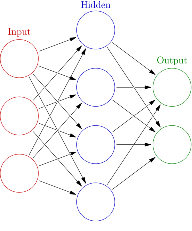
Figure 1: A schematic diagram of a fully connected three-layer feed-forward neural network, where each circle represents a neuron. Here, the data is fed into the input layer as an array, then transmitted to the hidden layer where it is mixed and reprocessed based on the weights of the connections leading into the hidden layer; the resulting values are sent to the output layer, where they are reprocessed one final time, ultimately producing a highly nonlinear model. [Glosser.ca]

Typically, neural networks contain many hidden layers, and thus possess an obscene number of parameters — in this paper, the authors use a network with 48,690,307 parameters! With this many parameters, neural nets run the risk of overfitting the data, using up a large amount of memory, and running extremely slowly. Fortunately, one can ameliorate these issues by adding one or more “convolution” layers to a network, filtering and contracting the data and preserving only the most salient features (for a more thorough explanation of this convolution process, see here); this is especially useful when processing detailed image data, such as the cosmic density maps that the authors use as their input data. The authors optimize their network by adopting a U-Net architecture, which employs a series of convolutions followed by a series of deconvolutions to quickly parse the input and highlight its key components.

To generate their training and testing data sets, the authors simulate the formation of large-scale structure up to the present day, retrieving both cosmic density and momentum maps; the density maps are used as inputs to the neural net, while the corresponding velocity maps — computed by dividing the momentum fields by the density fields — are used to evaluate the neural net’s output and to subsequently train, cross-validate, and test the resulting model.

Math vs. Machine

The authors assess the performance of their trained neural network by comparing its peculiar velocity predictions to those of linear perturbation theory. In nearly all cases, the neural net clearly outperforms the theoretical model. Perturbation theory performs well in regions of low density and velocity, occasionally yielding better predictions than the neural net. However, in regions of high density and velocity and in merger situations where two regions of opposing velocity collide with one another, perturbation theory fails completely, while the neural net still faithfully reconstructs the velocity field (see Figure 2). Over multiple testing data sets, the neural net is shown to be robust in all situations, while perturbation theory becomes practically useless in the presence of nonlinear dynamics.

six panel plot evaluating the neural net results

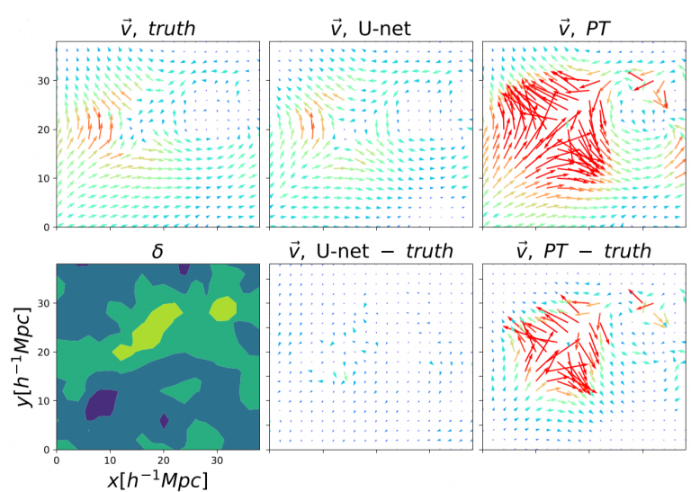
Figure 2: Comparison of a simulated velocity field (upper left) with a field predicted by the neural network (upper middle) and by perturbation theory (upper right); the lower left shows the underlying density field, while the lower middle and lower right show the residuals for the neural net predictions and the perturbation theory predictions, respectively. In regions of high density and velocity and in regions of converging flow, perturbation theory breaks down. [Wu et al. 2021]

While the neural network used in this paper can definitely be improved — perhaps by further optimizing its architecture or by using more training data — the authors have shown that neural nets can be valuable tools for predicting peculiar velocities. With such programs as DESI, EUCLID, the Rubin Observatory, and the Nancy Grace Roman Space Telescope promising to map out an unprecedented volume of the cosmos within the next decade, it is of utmost importance that we possess fast and accurate methods for parsing the new data — and neural networks are surely at the forefront of these methods. Maybe the rise of machines isn’t such a bad thing after all!

Original astrobite edited by Pratik Gandhi.

About the author, Ryan Golant:

I am a first-year astronomy Ph.D. student at Columbia University. My current research involves the use of particle-in-cell (PIC) simulations to study magnetic field growth in gamma-ray burst afterglows and closely related plasmas. I completed my undergraduate at Princeton University, and am originally from Northern Virginia. Outside of astronomy, I enjoy playing violin, studying art history, reading Wikipedia, and watching cat videos.

Spitzer photograph of a dramatic nebula surrounding bright point sources.

Editor’s note: Astrobites is a graduate-student-run organization that digests astrophysical literature for undergraduate students. As part of the partnership between the AAS and astrobites, we occasionally repost astrobites content here at AAS Nova. We hope you enjoy this post from astrobites; the original can be viewed at astrobites.org.

Title: The consistency of chemical clocks among coeval stars
Authors: Francisca Espinoza-Rojas et al.
First Author’s Institution: Pontifical Catholic University of Chile
Status: Submitted to ApJ

Stellar age is an extremely valuable parameter to constrain because it introduces time into our study of astronomical objects. Pairing the observed properties of stars with time opens up a rich new dimension in the study of our galaxy and beyond. For example, when we pair stellar age with stellar kinematics, we can dynamically trace stars back to their birth locations to study things like galactic evolution and star formation in detail. When we consider stellar age in our study of exoplanets, we can peer into the planet formation and evolution process. When we pair stellar age with stellar chemical abundances, we can trace the evolution of specific elements over time in the galaxy. Weaving time into these various analyses opens up a new realm of insight that enhances our understanding of the universe. However, with this all said, stellar age is extremely difficult to constrain.

Stellar Ages Are Hard to Determine

Some methods of constraining stellar ages include using photometry, dynamics, gyrochronology, and the abundances of individual elements like lithium in stars. For example, the locations of stars on the color–magnitude diagram (CMD), which are determined by photometry, can hint at stellar age. Many stellar and galactic astronomers fit isochrones, lines of constant age in the CMD, to the photometric data of a single or group of stars to estimate their age. However, this method relies on very well-constrained dust parameters between the observer and the object. Gyrochronology, using stellar rotation to estimate age, is another effective method, but it requires knowledge of the inclination of the star, something that is often difficult to determine. We can also use lithium abundances to estimate stellar age. Lithium, however, is only an effective age indicator in young stars with convective envelopes. As you can probably tell, there are tons of ways to estimate stellar age, but they all suffer from various limitations and uncertainties.

Abundance Ratios of Certain Elements Track with Age

An interesting, and somewhat new, avenue for probing stellar age is through the use of chemical clocks. Chemical clocks are sets of elemental abundance ratios that have been observed to track with stellar age. The idea behind chemical clocks is rooted in the notion that different families of elements are expelled into the interstellar medium (ISM) on different time scales (see Figure 1). For example, elements like Mg, Al, and Ti are produced in dying massive stars, which live short lives that end in core-collapse supernovae. As a result, these elements follow very different timescales than, say, Ba and Y — elements that are produced primarily in low-mass stars, which have much longer lifetimes and subsequently take longer to spread their nucleosynthetic products out into the ISM. This means that the ratios of various abundances in the ISM are constantly changing. When a star is born, it traps with it the chemical abundances of the ISM at the time of its birth like a time capsule and carries them with it throughout most of its life. Thus, the ratios of certain elements in a star could probe at what point in the Milky Way’s chemical evolution (and thus in time) the star was born.

diagram showing sources of chemical enrichment over time

Figure 1: A cartoon depicting the different timescales of chemical enrichment from various sources, the concept behind chemical clocks. Core-collapse supernovae, which come from short-lived massive stars, for example, dominate the chemical enrichment of the Milky Way early on. Asymptotic Giant Branch (AGB) stars, which originate from long-lived low- and intermediate-mass stars, start contributing to galactic chemical enrichment later on. [Jacobson & Frebel 2014]

Testing Chemical Clocks in Wide Binaries

The authors of today’s paper set out to investigate just how reliable chemical clocks are at keeping time by testing their consistency in wide binaries. Wide binaries are pairs of stars that were born together and orbit a common center of gravity. As their name implies, wide binaries have large separations, making them easier to study observationally. These systems are a great way to test chemical clocks because they consist of two stars that share an age. Today’s authors investigate various chemical clock abundance ratios in 36 pairs of wide binaries to see which chemical clocks are most consistent among stars born at the same time.

The authors are first able to recreate the result found in previous studies that wide binaries are more chemically similar in their elemental makeup than random pairs of stars in the field. This makes sense. Stars born in the same place should share the same chemical composition because the interstellar medium is understood to be very homogeneous on small spatial scales. The chemical abundances of stars directly reflect the chemical abundances of the material from which they were born, so if the interstellar medium is well-mixed, and stars share a birth place and age, then they should share a similar chemical profile.

42-panel plot exploring different abundance ratios among the binary pairs

Figure 2: The consistency in the abundance of various chemical clocks between both components of wide binaries. The x-axis in each subplot is the abundance in the indicated chemical clock for one component of the binary (A), and the y-axis is the same for the other component (B). The tighter the 1-to-1 relationship in a subpanel, the more consistent a chemical clock between stars in the binary pair. [Sc/Ba], [Al/Ba], and [Ti/Ba] (all in the 4th row), among others, stand out as chemical clocks that appear to be promising age indicators. [Espinoza-Rojas et al. 2021]

The authors then make an interesting discovery: when they investigate chemical clocks among wide binaries, they find that components of wide binaries tend to be even more similar in chemical clock abundances than other elemental abundances, as seen in Figure 2. They find that even when components of a wide binary are quite dissimilar chemically in [X/Fe], as is the case in one particular pair in their sample (black box in Figure 2), they are still very consistent in chemical clock abundances. This result suggests that chemical clocks could be effective age indicators even when stars are extremely dissimilar in other elements. The authors highlight that three chemical clocks in particular, [Sc/Ba], [Al/Ba], and [Ti/Ba], seem to be the most consistent among wide binaries and thus the most promising indicators of age.

What is next for the field of chemical clocks? One new avenue involves calibrating chemical clocks using stars with ages derived through other means, such as gyrochronology. This way, we can create an empirical, observed relationship between a star’s abundance in a chemical clock and its age. These empirical relationships will likely vary with Milky Way location, but they will open up a new avenue of probing stellar age in stars with a variety of parameters. With chemical clocks, we can hopefully expand our stellar age toolbox and allow for more checks on stellar age, an important parameter in observational astronomy.

Original astrobite edited by Lili Alderson.

About the author, Catherine Manea:

Catherine is a 2nd year PhD student at the University of Texas at Austin. Her research is in galactic archaeology, the practice of using the kinematic and chemical information of individual stars to study the evolution of our Milky Way. She is particularly interested in pushing chemical tagging, the practice of tracing stars back to their birth sites, to new limits.

Photograph of a galaxy undergoing ram pressure stripping

Editor’s note: Astrobites is a graduate-student-run organization that digests astrophysical literature for undergraduate students. As part of the partnership between the AAS and astrobites, we occasionally repost astrobites content here at AAS Nova. We hope you enjoy this post from astrobites; the original can be viewed at astrobites.org.

Title: ELVES I: Structures of Dwarf Satellites of MW-like Galaxies; Morphology, Scaling Relations, and Intrinsic Shapes
Authors: Scott G. Carlsten et al.
First Author’s Institution: Princeton University
Status: Accepted to ApJ

Dwarf galaxies are thought to be incredibly suggestible; there has been a range of diverse dwarf galaxies observed in our universe, indicating that they are extremely sensitive to their surroundings. The observed differences in sizes, shapes, and colours of dwarf galaxies is believed to be at least in part due to differences in the environment they inhabit. All galaxies are thought to be surrounded by a halo of dark matter (see this astrobite for more details). Many dwarf galaxies are satellite galaxies, meaning that they are found in orbit within a larger host dark matter halo that also typically contains a larger central galaxy (for example, the Small and Large Magellanic Clouds are satellite galaxies, both in orbit of our own Milky Way).

Satellite galaxies are subject to many different interactions with their host dark matter halo. These interactions between a satellite galaxy and its host can have devastating effects on the satellite galaxy itself. For example, their gas content can become extremely disturbed (and sometimes completely removed) by ram pressure stripping, which can eventually bring star formation in the satellite to a halt (see this astrobite for a summary of the seminal paper on ram pressure stripping). Similarly, their stars are subject to tidal stripping, which arises due to differences in the gravitational potential of the satellite galaxy and its host.

6-panel image showing photos of different types of dwarf galaxies

Figure 1: Examples of dwarfs visually classified as early-type (ETG) and late-type (LTG). Late-type dwarfs are irregular, with apparent active star formation throughout the galaxy while early-types are smooth and featureless without any star-forming clumps. [Carlsten et al. 2021]

Despite the observed diversity of dwarf galaxies, they can broadly be classified into two morphological types: late-type and early-type (see Figure 1 for examples). Late-type galaxies are typically star-forming, whereas early-type galaxies lack star-forming regions and appear smoother than late-types. Today’s paper uses the ongoing Exploration of Local VolumE Satellites (ELVES) Survey to investigate how the structural properties of dwarf galaxies can change depending on the environment and morphology of the galaxy. The galaxies in the ELVES sample are all within the Local Volume (D < 12 Mpc), and are satellite galaxies in orbit of Milky Way-like halos.

Going from a Late-type to an Early-type?

The current picture of dwarf galaxy evolution suggests that early-type dwarfs are formed from late-type dwarfs interacting with a host halo. If this is the case, then early-type dwarfs can be thought of as dwarf galaxies in the last throes of their evolution, and any differences in characteristics of late-type and early-type galaxies could provide insights into the physical mechanisms behind this evolution (such as the removal of star-forming gas through ram pressure stripping).

Plot of effective radius vs. log stellar mass for dwarf galaxies

Figure 2: Log effective radius vs. log stellar mass for the dwarf galaxies in the Local Volume sample. The upper panel displays points for each dwarf galaxy in the sample, with red indicating early-type and blue indicating late-type. The bottom panel shows average trends binned by stellar mass. The dashed lines show the mass-size relations for early-type (red) and late-type (blue) dwarf galaxies of higher stellar mass from the GAMA Survey. [Adapted from Carlsten et al. 2021]

To investigate whether there are any structural differences between early- and late-types, the authors plot the effective radius of the dwarf galaxies in their sample (essentially the galaxy’s size) by their stellar mass. It can be seen from Figure 2 that there is no significant difference between the early- and late-type galaxies at fixed stellar mass. This similarity between late-types and early-types suggests that the physical processes relevant in forming early-type galaxies (such as ram pressure stripping) do not necessarily induce any change in the galaxy’s size. These results indicate that the transformation process from late-type to early-type requires only the removal of the galaxy’s star-forming gas — significant structural change to the galaxy is not necessarily required. Also of note is the difference between the author’s results, where the sample is limited to dwarf galaxies with M* < 108.5 M and results for satellite galaxies with higher masses (indicated by the blue and red lines in the bottom panel of Figure 2). The authors suggest that this difference hints that there is a characteristic stellar mass scale, above which additional physical processes may be required to explain the sudden difference in sizes between early- and late-types.

Environmental Effects

The next question the authors aim to answer is: how does the mass of the dwarf galaxy’s host dark matter halo affect the evolution of the dwarf galaxy? To consider this, the authors again compare the sizes of dwarf galaxies. This time, a comparison is made between dwarf galaxies that are orbiting within larger cluster environments and the dwarf galaxies in their Local Volume environment.

Plot showing mass–size relations for cluster and field dwarf galaxies

Figure 3: The mass–size relations of the cluster (grey) and field (cyan) dwarf samples normalized to the full Local Volume sample (green). At fixed stellar mass, the cluster sample is offset to larger sizes, whereas the isolated field sample is offset to smaller sizes. Field galaxies are isolated dwarf galaxies that have been taken from an auxiliary sample, using additional observational data. [Adapted from Carlsten et al. 2021]

As can be seen in Figure 3, dwarf galaxies in cluster environments tend to be slightly larger than dwarf galaxies in the Local Volume at a fixed stellar mass. The authors argue that the observed increase in size is down to more intense tidal stripping and heating of galaxies in extreme cluster environments, which aligns with theoretical expectations. While an ~8% increase in sizes for the dwarfs in cluster environments is observed, the authors note the mass–size relation is strikingly similar between the two environments, especially since the mass of the host dark matter halos differ by a factor of 10. This is perhaps indicative that the exact environment plays a fairly small role in dwarf galaxy evolution — a somewhat surprising result!

In conclusion, today’s authors are able to gain insights into the physics of dwarf galaxy transformation from late-types to early-types, and how these processes vary between the Milky Way-like and cluster environments. The authors comment that a comparison with simulations will be useful in constraining the physics of how dwarf galaxies evolve. Their observational results have quantified the start and end points of the transformation, and simulations may now be able to tie them together to tell the middle part of the story!

Original astrobite edited by Luna Zagorac.

About the author, Katy Proctor:

I am a first-year PhD student at the International Centre for Radio Astronomy Research at the University of Western Australia. My research is focused on using cosmological simulations to study the evolution of satellite galaxies. Outside of research, I can usually be found climbing up walls or playing guitar.

Photograph of a blue planet

Editor’s note: Astrobites is a graduate-student-run organization that digests astrophysical literature for undergraduate students. As part of the partnership between the AAS and astrobites, we occasionally repost astrobites content here at AAS Nova. We hope you enjoy this post from astrobites; the original can be viewed at astrobites.org.

Title: Eccentric Early Migration of Neptune
Authors: David Nesvorný
First Author’s Institution: Southwest Research Institute
Status: Published in ApJL

Among the furthest reaches of our solar system, beyond the orbits of the mighty ice giants, lies the Kuiper Belt. This circumstellar disk, roughly twenty times as wide as the asteroid belt, is home to many small bodies (defined by the IAU as any Sun-orbiting body that is neither a planet, dwarf planet, nor satellite), as well as various dwarfs, including what was once the ninth planet. Collectively, these bodies are referred to as Kuiper Belt Objects (KBOs), which are themselves a subset of Trans-Neptunian Objects (TNOs). Understanding the collective orbits of KBOs provides important insights into the evolutionary history of our early solar system.

Neptune, like other outer gas giants, is known to have migrated in the past and interacted with KBOs. We can predict what Neptune’s migratory orbit was like by simulating different planetary migration scenarios for the outer planets, seeing how they affect KBOs, then finding the parameters that best match currently observed KBO orbits. Today’s paper examines a group of KBOs within a specific range of orbital parameters whose current orbits are unable to be accounted for in simulations if Neptune migrated with a low orbital eccentricity (<< 0.03). Instead, better results are obtained if Neptune migrated with a higher eccentricity of e ~ 0.1.

Space For The Travelling Planet

Under the current framework for accounting for the dynamical evolution of the early solar system, Neptune is known to have migrated into a higher orbit, subsequently interacting with the Kuiper Belt and its various KBOs. After this migration, Neptune’s orbit slowly decayed and circularised, causing the planet to move inward to its current position today. This migration is noted to have altered the distribution of inclinations and eccentricities of KBOs, and (in conjunction with other migrations by Uranus, Saturn, and Jupiter) is theorised to be responsible for scattering many KBOs and other planetesimals into the inner solar system (the Late Heavy Bombardment). Studies focusing on this period of instability have aimed to constrain the eccentricity of Neptune’s migration. There are many factors to consider, such as tidal interactions and possible orbital resonances with KBOs or the other gas giants, dynamical friction, and Kozai cycles (which cause eccentricity and inclination to oscillate).

This study definitively rules out the low-eccentricity migration scenario, and instead provides support to an excitation scenario wherein Neptune had an eccentricity of e ~ 0.1.  The data used to fine-tune the simulations was obtained from the Outer Solar Systems Origin Survey (OSSOS), which identified a population of KBOs with semimajor axes between 50 and 60 AU, a perihelion distance greater than 35 AU, and an inclination of less than 10 degrees. Figure 1 shows all KBOs with semimajor axes between 50 and 60 AU plotted by eccentricity, with the OSSOS samples highlighted as blue triangles. Simulations show that the existence of this population is easily accounted for in the high-eccentricity model; here bodies originally at around 30 AU are scattered into higher orbits (50 to 60 AU), where they subsequently interact with Neptune due to mean motion resonances. The bodies eventually decouple, forming the specific 50–60 AU population that we see today.

Plot showing eccentricity vs. semimajor axis for KBOs

Figure 1: A plot of modelled orbits of KBOs with semimajor axes between 50 and 60 AU plotted by eccentricity (shown as red dots), with the OSSOS detections overlaid as blue triangles. [Nesvorný 2021]

A Wandering Neptune

Importantly, this study provides a key physical explanation as to why the low-eccentricity model cannot work in practice. Were Neptune to have a low eccentricity, the mean motion resonances would not be as effective, and so the scattered KBOs would need to decouple via Kozai resonances. However, in Kozai cycles, as eccentricity decreases, inclination must increase. The KBOs in this situation would thus be unable to satisfy the target parameter range of having less than 10 degree inclination (see Figure 2, which shows this exclusionary zone). The only other explanation for their existence is that these KBOs originated in situ, in some hypothetical disc that was perturbed by other means.

2-panel plot of inclination vs. perihelion distance for KBOs under 2 models.

Figure 2: Orbital inclinations and perihelia for KBOs with semimajor axes between 50 and 60 AU. Left and right panels correspond to two different dynamical models. Blue triangles denote the OSSOS samples. The olive shaded region is the excluded region in which objects scattered by a low-eccentricity Neptune cannot exist. The fact that OSSOS samples do exist rules out the low-eccentricity case. [Nesvorný 2021]

Questions remain over the exact cause of Neptune’s high-eccentricity migration in the first place. One scenario involves a mean motion resonance between Uranus and Neptune, but it is rare for such effects to alter eccentricity by the degree required (of order 0.05). Comparatively, encounters with Saturn and Jupiter do have the potential to propel Neptune into a highly eccentric orbit (of order 0.2), but such scenarios do not reconcile with KBO observations. Instead, the most likely scenario is that Neptune had an encounter with a rogue planet. Such a planet would need to have been at least as massive as the Earth, though detailed predictions of possible trajectories are, as yet, unable to be gleaned from the current KBO population nor from simulations. That said, based on the current KBO population, it is possible to estimate how many Earth-like planets could have been in the outer solar system; one study gives an 68% likelihood of fewer than 3.

And Yet They Moved

The Kuiper Belt remains an active frontier for research into the dynamical evolution of the early solar system. Not only does accounting for the orbital properties of KBOs yield insights into the evolutionary history of the outer planets, but it enhances our understanding of the physical processes at play — from mean motion resonances to Kozai cycles — allowing us to better constrain the orbital parameters of migrating planets. This is important given the rise of exoplanetary science, and the need to account for the many exotic planetary configurations that have been discovered. Only then can we build a complete picture of how planetary migration affects planetary systems.

Original astrobite edited by Gloria Fonseca Alvarez.

The author would like to acknowledge the Whadjuk peoples of the Noongar nation, the traditional custodians of the land on which this post was written, and pays respects to Elders past and present.

About the author, Mitchell Cavanagh:

Mitchell is a PhD student in astrophysics at the University of Western Australia. His research is focused on the applications of machine learning to the study of galaxy formation and evolution. Outside of research, he is an avid bookworm and enjoys gaming, languages and code jams.

Photograph of a false-colored bright green nebula.

Editor’s note: Astrobites is a graduate-student-run organization that digests astrophysical literature for undergraduate students. As part of the partnership between the AAS and astrobites, we occasionally repost astrobites content here at AAS Nova. We hope you enjoy this post from astrobites; the original can be viewed at astrobites.org.

Title: Magnetic Fields and Star Formation Around HII Regions: The S235 Complex
Authors: R. Devaraj et al.
First Author’s Institution: Dublin Institute for Advanced Studies, Ireland
Status: Published in ApJ

Massive young stars heat the interstellar material around them, creating HII regions, or areas full of ionized hydrogen. As the stars push stellar wind and ultraviolet radiation outward, their HII regions expand, and a balloon of interstellar material begins to collect around the central star. Surrounding gas and dust is swept up by the balloon, and the magnetic field changes.

Astronomers know that magnetic fields play an important role in star formation. And we also know that expanding HII regions can trigger star formation. But how the two fit together in the overall process of creating new stars remains mysterious. Today’s paper examines S235, a star-forming complex that is home to HII regions and young stellar objects, in order to explore how the magnetic field structure and strength affects star formation.

The Balloons In Star-Forming Complex S235

S235 contains three HII regions, which are labeled in Figure 1 as S235 Main, S235AB, and S235C. The star symbol shows the central ionizing star for S235 Main, while the crosses show the same for the smaller HII regions. Past studies have identified many young stellar objects (YSOs) in this field. The white dashed boxes show where clusters of those baby stars are located. Many of the YSOs are located right on the edge of the largest inflating, balloon-like HII region.

Infrared photo of a nebula with different regions outlined and labeled.

Figure 1: The S235 field of view in the infrared. There are three HII regions, which are seen as the pink, roughly circular structures. Each has a central ionizing star. Clusters of young stellar objects are traced in the white dashed rectangles. [Devaraj et al. 2021]

Polarization Traces Inflation

The authors of today’s paper used polarimetry from the Mimir and POLICAN instruments to trace the magnetic field in this complex. Near infrared polarimetry measures the orientation of light from stars in the background. Egg-shaped dust grains in the interstellar medium will align their long axes perpendicular to magnetic fields, which means the dust blocks one orientation of light more than another. By measuring that orientation, we trace the magnetic field!

It’s important to make sure that the polarization measurements used in this study are actually behind the HII regions; otherwise, they aren’t examining the magnetic field in the right place. The authors filtered out foreground stars using Gaia distances and constraints on the extinction, or the amount of dust that must be present towards a star. They also threw out the polarization data from young stellar objects, which create their own polarization from their circumstellar disks.

In order to get rid of any foreground dust component, the authors subtracted the average polarization of the foreground stars from the stars in the background, which left them with the orange polarization vectors shown in Figure 2. The direction of the vectors traces the magnetic field, while their length shows the strength of the polarization. It’s pretty clear that for S235 Main, the magnetic field traces the outskirts of the HII region! That means the magnetic field is pushed and compressed as the HII balloon inflates.

Infrared photo of a nebula with magnetic field vectors overplotted.

Figure 2. Polarization measurements for stars behind the S235 complex. The vectors trace the magnetic field, which appears to follow the outskirts of the largest HII region bubble. [Devaraj et al. 2021]

Clumpy Clouds Created Stars

Using maps of gas and dust intensity, today’s authors also identified 11 main clumps of interstellar material in the field of view. They measured the magnetic field strength in those clumps and found that the magnetic energy was dominant over both turbulence and gravity. The magnetic field is actually so important that it has slowed star formation, bringing it to a halt.

But the presence of YSOs means that star formation had to have happened at some point in the past. The authors suggest a timeline of events: 1) Before the HII region expanded, the magnetic fields and gravity balanced out, creating an equilibrium. 2) As the HII region began to expand, it created dense regions and turbulence, which caused the gas and dust to collapse and stars to form. 3) The turbulence decayed and the magnetic field became more important. It started regulating and stopping star formation, leading the region to look how it does today.

This new understanding of how magnetic fields and HII regions are related is crucial to compiling an overall picture of star formation. But the overall process is complicated and involves so many moving parts that there is still much to be learned about how stars are born!

Original astrobite edited by Ciara Johnson.

About the author, Ashley Piccone:

I am a third year PhD student at the University of Wyoming, where I use polarimetry and spectroscopy to study the magnetic field and dust around bowshock nebulae. I love science communication and finding new ways to introduce people to astronomy and physics. In addition to stargazing at the clear Wyoming skies, I also enjoy backpacking, hiking, running and skiing.

False-color photograph showing wispy molecular clouds in a space field.

Editor’s note: Astrobites is a graduate-student-run organization that digests astrophysical literature for undergraduate students. As part of the partnership between the AAS and astrobites, we occasionally repost astrobites content here at AAS Nova. We hope you enjoy this post from astrobites; the original can be viewed at astrobites.org.

Title: The Single-Cloud Star Formation Relation
Authors: Riwaj Pokhrel et al.
First Author’s Institution: University of Toledo
Status: Published in ApJL

Gas to Stars

Photograph of a dark cloud in the midst of a wispy nebula.

A Hubble view of a molecular cloud, roughly two light-years long, that has broken off of the Carina Nebula. [NASA/ESA, N. Smith (University of California, Berkeley)/The Hubble Heritage Team (STScI/AURA)]

Each of the many hundreds of stars we can see with our naked eye, or the many thousands we can see with the aid of telescopes, has their own special story of how they came to be. Now self-gravitating balls of gas, these stars in the night sky began as clumps in dense molecular clouds. Once these clumps become large enough, they gravitationally collapse and form stars. In our own galaxy, the Milky Way, we can study this process directly and use the observations to infer much about its workings in more distant galaxies.

Since we know that dense gas is required to form stars, it is natural to ask what relationship there is between the two. In fact, the Kennicutt–Schmidt (KS) relation tells us that there is a direct scaling between the mass of gas and the star formation rate (SFR). This relationship has allowed us to trace star formation throughout the history of the universe and understand how galaxies grow over cosmic time. But the authors of today’s paper asked a question that puts a slight twist on the KS relation: they wanted to know if such a relationship holds within individual molecular clouds.

Putting Clouds Under the Microscope

To answer this question, the authors used Spitzer and Herschel data for 12 well-studied star forming regions. Using the Herschel far-infrared data, they computed molecular hydrogen column density maps. With these measurements, they were able to compute the surface density of the gas in the star forming regions. With both near- and mid-infrared data from Spitzer the authors identified sources with a significant infrared excess and classified them into subclasses of young stellar objects (YSOs), also known as protostars. With these data, the authors measured the gas masses and number of stars within given density contours (corresponding to a physical area in the cloud). Figure 1 shows these values. From these, a gas surface density, a star formation surface density, and a free-fall timescale can be calculated. The authors assumed a stellar mass of 0.5 solar mass and a 0.5-Myr timescale to compute the SFR.

two plots indicating that strong correlation exists between the number of protostars and the gas column density.

Figure 1: A strong correlation exists between the number of protostars and the gas column density. Top panel: Gas column density map of the Mon R2 molecular cloud. The brown contours indicate lines of constant surface density and the magenta stars are identified protostars. Bottom panel: Molecular gas mass (circles) and the number of protostars (diamonds) within each contour. [Pokhrel et al. 2021]

The Single Cloud Relation

With measured gas and SFR surface densities, the authors were ready to answer their main question. Figure 2 shows the comparison of these two quantities. As can be seen, the SFR surface density and the gas surface density scale strongly with each other. In fact, when normalizing by the free-fall timescale (right panel of Figure 2), the scatter in the relationship is decreased and the relationship becomes linear, as expected from theory.

plots showing the gas and SFR surface densities are highly correlated.

Figure 2: The gas and SFR surface densities are highly correlated. The above plot shows log of the SFR surface density as compared to the log of the gas surface density (left panel) and gas surface density divided by the free-fall time (right panel). The black line is the median best-fit relation and the dark and light gray shaded regions show one and two standard deviations from the fit respectively. [Pokhrel et al. 2021]

To further demonstrate that the relationship shown in Figure 2 is real and not due to the fact that both surface densities are area-dependent, the authors compare the gas surface density to the free-fall efficiency, which essentially measures how efficient the gas is at forming stars on a free-fall timescale. This comparison is shown in Figure 3. With no clear global trend between the free-fall efficiency and the gas surface density, the authors are confident that their single cloud star formation relationship is valid.

plot of free-fall efficiency vs. gas surface density.

Figure 3: The gas surface density and free-fall efficiency are uncorrelated, suggesting the above relationship is real. The above plot shows log of free-fall efficiency as compared to the log of the gas surface density. The median log free-fall efficiency is shown by the black line. [Pokhrel et al. 2021]

In summary, the authors of today’s paper have shown that the KS relation that has been used for years in extragalactic studies has a local analog. This is particularly interesting as the various clouds in their sample have a wide range of physical properties. This correlation implies that star formation is regulated by processes on small scales, including stellar outflows or turbulence, rather than galaxy-scale effects such as supernovae and galactic properties. As we continue to study star formation in greater detail, the deeper meaning of this correlation may give us even deeper insights into how the stars we see every night were born.

Original astrobite edited by Suchitra Narayanan.

About the author, Jason Hinkle:

I am a graduate student at the University of Hawaii, Institute for Astronomy. My current research is on multi-wavelength photometric and spectroscopic follow-up of tidal disruption events. My research interests also include a number of topics related to AGN, including outflows, X-ray spectroscopy, and multi-wavelength variability. In addition to my love for astronomy, I enjoy hiking, sports, and musicals.

Illustration of a dark body in the distant outer reaches of the solar system.

Editor’s note: Astrobites is a graduate-student-run organization that digests astrophysical literature for undergraduate students. As part of the partnership between the AAS and astrobites, we occasionally repost astrobites content here at AAS Nova. We hope you enjoy this post from astrobites; the original can be viewed at astrobites.org.

Title: Injection of Inner Oort Cloud Objects Into the Distant Kuiper Belt by Planet Nine
Authors: Konstantin Batygin and Michael E. Brown
First Author’s Institution: California Institute of Technology
Status: Accepted to ApJL

Ladies and gentlemen, welcome aboard the Astrobites Airlines with service from the Earth to Planet Nine. We are currently fourth in line for take-off, but you can learn more about other take-offs to Planet Nine here, here, and here. We are traveling at the speed of light and the duration of our flight will be about 70 hours. We ask that you please enjoy our long journey to the outer solar system.

Diagram illustrating the locations of the Kuiper Belt and the Oort cloud in our solar system.

Figure 1: The Kuiper Belt and Oort Cloud location. [ESA]

Our journey starts in the Kuiper Belt, a ring of icy bodies residing beyond Neptune’s orbit. Look around — these are distant Kuiper Belt Objects (KBOs) (look at Figure 1)! We can see (also in Figure 2) two distinct types of distant KBOs: some KBOs have dynamically stable orbits and some do not. Those that are unstable are destabilized by Neptune. The observed clustering of stable orbits needs to be affected by something so that it maintains orbital alignment against differential precession induced by Jupiter, Saturn, Uranus, and Neptune (huge planets that have huge gravity!). So, what is affecting the orbits of the stable KBOs? The authors of today’s paper think it could be Planet Nine!

Schematic showing the orbits of a set of distant Kuiper Belt Objects

Figure 2: Census of distant KBOs. The orbits of stable KBOs are depicted in purple and grey. Unstable ones are depicted in green. [Batygin & Brown 2021]

We Forgot That the Universe Is BIG!

The authors have been working on Planet Nine for a long time (their first paper hypothesizing the existence of this distant, unseen giant planet in our solar system was published in 2016)! During this time, they made some estimates on dynamical properties of the planet we are heading to right now. For example, Planet Nine might have a mass of 5 Earth masses, with a semi-major axis of 500 au, an eccentricity of 0.25, and an inclination of 20 degrees from the data that was observed (Planet Nine itself has not yet been observed). However, all this time, the authors treated the solar system as an isolated object, neglecting all the bodies that attain a heliocentric distance of over 10,000 au. But these bodies are still there! The authors’ assumption is valid for representing the evolution of objects with semi-major axes on the order of a few hundred au. More recent detections of trans-Neptunian objects (TNOs), however, increasingly point to a pronounced abundance of long-period TNOs with a heliocentric distance of over 10,000 au. This orbital domain borders the inner Oort cloud (IOC). More importantly, the population of debris in the IOC is stable, just like the KBOs mentioned above! So, the authors’ hypothesis is that some of these stable KBOs were injected into the Kuiper Belt from the outside, possibly due to the influence of Planet Nine.

The Tug-of-War Between Giant Planets and Stars

As we go further and further from the Sun on our spaceship, it is important to note that the Sun’s birth environment played an important role in shaping the solar system. After all, the Sun is the reason we have our solar system in the first place! The Sun, like any other star, was born in a big family of stars — a cluster. Now, it’s time to wear your glasses, because it’s simulation time!

The authors made an N-body simulation of the formation of our solar system including Jupiter and Saturn (they are significant because they are huge) and 100,000 planetesimals, spanning the 4.5−12 au range in the heliocentric distance in initial circular and coplanar orbits. They modeled the Sun’s birth cluster as a Plummer sphere. The Plummer sphere is often used in N-body simulations to “soften” gravity at small distance scales. This is needed to prevent the point particles from scattering too strongly off of one another on a close approach. Along with Jupiter and Saturn, they also modeled “passing stars” — members of the Sun’s family that might have affected the debris gravitationally. All of it, the concurrent growth of giant planets and the passing stars, affects the planetesimals. Think of it as a tug-of-war between Jupiter and Saturn on one side and the passing stars on the other side. Because these icy objects (a.k.a. planetesimals) don’t know where to go, they choose to “freeze” in place, thousands of au away from the Sun. These are what the IOC is formed of.

Have We Reached Planet Nine Yet?

Dear passengers, it’s the time for another simulation! In absence of Planet Nine, the IOC created by the tug-of-war between giant-planet scattering and the passing stars would essentially remain dynamically frozen over the main-sequence lifetime of the Sun. But that’s because Planet Nine wasn’t considered in the first simulation. Let’s see what happens when the authors add Planet Nine.

In this simulation, the authors accounted for the dynamics driven by Neptune, Planet Nine, and the passing stars as well as the effect of the galactic gravitational tidal field and the average effect of Jupiter, Saturn, and Uranus. They found that over the lifetime of the Sun, a significant fraction (that is, on the order of 20%) of the IOC gets injected into the distant Kuiper belt. The authors also found that these re-injected IOC objects exhibit orbital clustering, which is important for the Planet Nine hypothesis (see this previous bite for more details). However, the degree of clustering is considerably weaker. The data suggests that Planet Nine might be even more eccentric than we thought. So, our journey might take a little longer! Another key result of the simulation is that IOC objects display a very extended semi-major axis distribution, which might explain objects like the Goblin.

Three scenes modeling the simulated evolution of the solar system, illustrating body orbits.

Figure 3: Sequence of events modeled within this work. A population of trans-Neptunian objects forms while the Sun is still in its birth cluster. Subsequently, over the billion-year lifetime of the solar system, Planet Nine slowly affects these extremely long-period objects, mixing them into the observed census of Kuiper belt objects. [Batygin & Brown 2021]

We are happy that you chose us again for your journey. We are really excited to see what is really out there, far away in our solar system. Thank you for choosing Astrobites Airlines!

Original astrobite edited by Catherine Manea.
A Russian translation of this article is available on Astrobites, also written by Sabina Sagynbayeva.

About the author, Sabina Sagynbayeva:

I’m a graduate student at Stony Brook University and my main research area is planets. I’m currently working on planet formation using hydrodynamical simulations. I’m mainly interested in planet-disk interaction but nearly any topic related to planets is fascinating to me! In addition to doing research, I’m also a singer-songwriter. I LOVE writing songs, and you can find them on any streaming platforms.

An artist's impression of a rocky exoplanet is seen in the centre of the image, illuminated from the right by a large star. The planet is dark, almost black in colour, however small cracks cover its surface revealing glowing red underneath, as if the planet is made of magma that has cooled in places. The planet's atmosphere appears to be being blasted away from the planet by the star.

Editor’s note: Astrobites is a graduate-student-run organization that digests astrophysical literature for undergraduate students. As part of the partnership between the AAS and astrobites, we occasionally repost astrobites content here at AAS Nova. We hope you enjoy this post from astrobites; the original can be viewed at astrobites.org.

Title: Water On Hot Rocky Exoplanets
Authors: Edwin S. Kite, Laura Schaefer
First Author’s Institution: University of Chicago
Status: Published in ApJL

Most Sun-like stars are thought to be home to a hot rocky exoplanet — which could mean that there are more than 300 million potentially habitable planets in our galaxy! However, whether any of these planets have atmospheres remains unknown. Unlike the Blue Marble we call home, the way that many of these planets form leaves them as dead rocks.

Most terrestrial planets larger than Earth (known as super-Earths) are thought to form as sub-Neptunes, consisting of a silicate magma ball surrounded by a thick atmosphere accreted from the planetary disc during formation. Because this atmosphere is dominated by light hydrogen molecules, it has a low mean molecular weight (µ, the average weight of each molecule in the atmosphere) and is later lost to space via atmospheric escape, leaving behind the bare super-Earth. While it’s possible for planets to later regain an atmosphere via volcanic activity or impacts from comets, what if there were a way for super-Earths to develop atmospheres while they evolve from sub-Neptunes?

Today’s paper explores a potential pathway that can not only generate super-Earth atmospheres, but could also allow them to be retained for billions of years.

When Magma Meets Air

The authors consider what happens to the products that form when a sub-Neptune’s magma reacts with its atmosphere. Iron oxides in the magma react with the atmospheric hydrogen, producing water, and iron, which sinks to the planet’s core. While some of this steam escapes into the atmosphere and mixes with the hydrogen, most of it dissolves and remains trapped in the magma, creating a planet made up of a slightly watery magma ball surrounded by a slightly higher-mean-molecular-weight atmosphere. But as the atmosphere begins to escape, what happens to the water?

diagram titled "pathways to a high-molecular-weight atmosphere"

Figure 1: A graphical representation of the potential pathways a sub-Neptune can take to become a super-Earth with a high-mean-molecular-weight (µatm) atmosphere. Blue atmospheres are hydrogen dominated, while green atmospheres are water dominated. The left-hand side shows a sub-Neptune losing its atmosphere to space, becoming a bare rock, and later regaining a high-µatm atmosphere. The right-hand side shows the pathway outlined in today’s paper, with a sub-Neptune evolving to a super-Earth with a water-dominated atmosphere via atmosphere–magma interactions. In each pathway, the sub-Neptune moves across the radius valley, decreasing in radius as it goes. [Adapted from Kite & Schaefer 2021]

Using models of planets, the atmospheres of each planet are removed in small steps, reassessing the equilibrium between the magma and the atmosphere each time. With each step, the pressure at the surface of the magma decreases, allowing some of the gases trapped there to escape. As the atmospheric loss continues, the model atmosphere gets thinner and thinner, while the large reservoir of water dissolved in the magma continues to be released. As outlined in Figure 1, over time the hydrogen will be completely lost, leaving behind a 150–500 km thick atmosphere and a water-dominated world! This kind of watery atmosphere can be referred to as being endogenic, as it originates from within the planet, as opposed to the exogenic atmospheres created by external processes, like being hit by an icy comet.

Water, Water, Everywhere?

The length of time for which a planet has a water-dominated atmosphere depends on how aggressive the atmospheric loss is. While smaller planets very close to their stars are at higher risk for atmospheric loss, planets at greater distances from their stars are safer and may never endure the process. Planets in between these extremes are able to keep hold of their newly acquired water-dominated atmospheres for varying lengths of time, but could potentially retain them for billions of years. So which planets can we expect to have watery envelopes?

When plotted on a graph of planetary radius vs. orbital period, the larger-radius sub-Neptunes and smaller-radius super-Earths are separated by a lack of planets often known as the radius valley. As a sub-Neptune loses its atmosphere its radius decreases, moving it down through the radius valley. The authors predict that, provided the planet has a long enough period and the interactions between magma and atmospheres are sufficiently efficient, the evolving planets that are able to retain water-dominated atmospheres should be found lining the radius valley in a “water belt”, as seen in Figure 2.

A plot of radius vs period showing planets near the radius valley

Figure 2: The “water belt” of super-Earths, shown in period–radius space for planets orbiting stars less than 3 Gyr old. The blue region shows the area occupied by sub-Neptunes, while the red region shows the area occupied by super-Earths. The yellow region in between is known as the radius valley. The water belt, where super-Earths with water dominated atmospheres may exist, is shown in green. The upper and lower dashed lines give the water-belt predictions for magmas with lower and higher amounts of iron oxides present. [Kite & Schaefer 2021]

Testing whether such planets exist could be relatively straight forward. Directly detecting the atmosphere of this kind of planet may be possible using a phase curve — a measurement of the light reflected and blocked by a tidally locked planet as it passes behind and in front of its host star. If the planet has retained the watery atmosphere, then heat can be more effectively distributed from the permanently illuminated day side to the cold, dark night side, leading to a smaller temperature difference between the two faces than would be the case for a bare, atmosphere-free rock. As endogenic atmospheres are likely to have smaller carbon-to-oxygen ratios than those on other super-Earths, observing the spectroscopic features of these atmospheres with the upcoming James Webb Space Telescope could also help distinguish between the two!

Original astrobite edited by Huei Sears.

About the author, Lili Alderson:

Lili Alderson is a first year PhD student at the University of Bristol studying exoplanet atmospheres with space-based telescopes. She spent her undergrad at the University of Southampton with a year in research at the Center for Astrophysics | Harvard-Smithsonian. When not thinking about exoplanets, Lili enjoys ballet, film and baking.

K2-18b

Editor’s note: Astrobites is a graduate-student-run organization that digests astrophysical literature for undergraduate students. As part of the partnership between the AAS and astrobites, we occasionally repost astrobites content here at AAS Nova. We hope you enjoy this post from astrobites; the original can be viewed at astrobites.org.

Title: Finding Signs of Life in Transit: High-resolution Transmission Spectra of Earth-like Planets around FGKM Host Stars
Authors: Lisa Kaltenegger, Zifan Lin
First Author’s Institution: Cornell University & Carl Sagan Institute
Status: Published in ApJL

Anybody Out There?

One of the most fascinating topics in astronomy — and maybe in philosophy, as well — is the potential existence of other life out there in space: strange planets orbiting other stars, developing and evolving their own biology under unique circumstances.

Fortunately, life leaves so-called biosignatures for the keen observer to find; these biosignatures should be most prominent in the atmosphere of an inhabited planet. The presence of certain substances and molecules in an atmosphere suggests biological processes indicative of life. For instance, life creates large amounts of molecular oxygen (O2) by photosynthesis and small amounts of methane (CH4) on Earth. The simultaneous presence of these two molecules are strongly suggestive of biological processes, since on short timescales, these two species react to create carbon dioxide (CO2) and water (H2O) and must therefore constantly be replenished to remain detectable. The same goes for ozone (O3), which, if not replenished, decays into O2 within days. Water is often mentioned as an important secondary indicator for life as well as carbon dioxide. On their own, these molecules are not decisive, however in combination they can paint a clearer picture.

transmission spectroscopy

Figure 1: As a star’s light filters through a planet’s atmosphere on its way to Earth, the atmosphere absorbs certain wavelengths depending on its composition. [European Southern Observatory]

If a system is favorably inclined relative to an observer, stellar light passing through the exoplanet’s atmosphere can be analyzed after careful data reduction and calibration by spectroscopy; this is illustrated in Figure 1. The elements and molecules present in the atmosphere reveal themselves in the form of spectral lines and allow for a substantial analysis of the atmospheric composition.

New telescopes, such as the JWST and the ELT, make this highly detailed, so-called transmission spectroscopy possible. But where should we look to maximize our chances of actually finding life?

Simulating Biosignatures

The authors of today’s paper simulated the spectra of 12 Earth-like planets around FGK stars (between about 1,900 Kelvin cooler and 1,200 Kelvin hotter than the Sun) and 10 M dwarfs (about 1,900 Kelvin to 3,300 Kelvin cooler than the Sun) to a level of detail that will be achieved with upcoming spectrographs. In this way, researchers can prioritize exoplanets for atmospheric investigation, according to the expected signal strength of the biosignatures.

To conduct this simulation, a model is required. It takes into account the planet, its location, and any processes we know of that influence its atmosphere.

The habitable zone is largely defined by conditions that make liquid water possible. For the purposes of this work, the temperature on the simulated Earth-like planets was set to 288 Kelvin +/- 2%. To maintain this temperature, different stellar types have their habitable zones at different radial distances. Thus, a habitable planet around an M dwarf is much closer to its host star than a similar planet around a F star.

In terms of the simulated planet’s architecture, the authors decided to model the planets using Earth-like properties. The planets were simulated to have one Earth-radius, one Earth-mass, and similar rates of irradiance, outgassing, composition (70% ocean and 30% land made from basalt, granite, sand, grass, trees, and snow), surface pressure, and cloud coverage relative to modern Earth.

Now, let’s talk about our biosignature pairs O2+CH4 and O3+CH4. Ozone layer depth decreases for lower ultraviolet (UV) light environments, since it is this radiation that splits up O2 in the atmosphere, so that the two halves may combine with other O2 molecules and build O3. On the other hand, methane concentration increases with lower UV radiation since the molecules that methane reacts with on Earth are indirectly created with the help of UV light.

However, methane may be reduced by so-called space weather. This includes stellar activity, such as flares or stellar winds which send out charged particles at the planets, which then interact with the atmospheres. It is thus important to check the surroundings of the planet when searching for life on it, since non-biological environmental factors can be responsible for additionally increasing or decreasing biosignatures.

How Deep Can You Go?

The authors divided up the planetary atmospheres into 52 layers and simulated the width and strength of the spectral lines for each. There is a limit to the depth an observer may look into an atmosphere, since deeper layers deflect the light. Earth’s atmosphere, for example, could be probed to around 13 km above ground. Depending on the stellar type and thus the predominant wavelengths emitted by the star (shorter wavelengths coming from hotter stars are refracted more severely than the longer wavelengths emitted by cooler stars), planetary atmospheres can be probed to between 15.7 km (for planets orbiting F0V type stars) and 0 km (for planets orbiting M8V type stars) above their surface.

Clouds can heavily obscure spectral features of the layers below them. Because we do not know any details about cloud coverage on exoplanets, the authors included hypothetical spectra considering a 100% cloud coverage at a height of 6 km (the altitude of the middle layer of Earth clouds). This only affects the efficiency of detecting biosignatures for planets around M type stars, since they can theoretically be probed below this altitude.

Who Shows Their True Colors?

The overall strength of a spectral feature is determined by its abundance in an atmosphere, as well as the maximum depth an atmosphere can be probed to during a transit. The resulting simulated spectra are shown in Figure 2.

CO2, water, and oxygen show similar signal strengths across all modeled atmosphere spectra, however for water and oxygen, the detectability is strongly dependent on the maximum probable depth due to their location at relatively low altitude. Thus, these features on an Earth-like planet around a hot F-type star would be extremely difficult to find.

Stars with increased UV radiation (F types as well as active M dwarfs) show a high abundance of ozone in their planets’ atmospheres. Methane features can be best detected on planets in orbit around cooler stars with lower UV environments.

set of 12 plots showing simulated transmission spectra

Figure 2: Transmission spectra simulated by the authors for Earth-like planets hosting life in orbit around F stars (top row), G stars (second row), K dwarfs (third row), and M dwarfs (bottom row). The three columns display different wavelength ranges, from visible (left) through near-infrared (middle) to infrared (right) light. The most prominent spectral features are labeled with the names of their corresponding molecules. [Kaltenegger & Lin 2021]

Hence, the authors have shown that the biosignature pairs O2+CH4 and O3+CH4 become increasingly difficult to find in planets orbiting hotter stars. A potential way to increase methane levels would be to use a younger Earth model, when methane levels were much higher than in modern times. If we want to look for life around hotter stars, it could be feasible to search in younger systems where detection of methane may be more likely.

The highly detailed simulation conducted by the authors will be an excellent tool to prioritize systems to search for life. With thousands of exoplanets already confirmed, this may prove vital in conducting efficient searches and will maybe one day allow us to look upon our night sky and point to the one little, insignificant dot that we then know illuminates someone else’s home.

Original astrobite edited by Katy Proctor.
A German translation of this article is available on Astrobites, also written by Jana Steuer.

About the author, Jana Steuer:

I’m a second year PhD student at the LMU Munich, working for the University Observatory (USM), which owns the 2.1m Fraunhofer Telescope Wendelstein. My field of research is exoplanets. I hunt for traces of them in data from big surveys, like the TESS mission and then follow them up, using spectroscopy and photometry. Mainly, I focus on long period planets that may potentially harbor life. When I’m not planet hunting, I act as a DM for several Dungeons and Dragons groups and annoy people with facts from Tolkien’s Silmarillion. I enjoy kickboxing and learning about ancient human history.

Three images of M87 at different wavelengths

Editor’s note: Astrobites is a graduate-student-run organization that digests astrophysical literature for undergraduate students. As part of the partnership between the AAS and astrobites, we occasionally repost astrobites content here at AAS Nova. We hope you enjoy this post from astrobites; the original can be viewed at astrobites.org.

Title: Broadband Multi-wavelength Properties of M87 during the 2017 Event Horizon Telescope Campaign
Authors: The Event Horizon Telescope Multi-wavelength Science Working Group
First Author’s Institution: N/A
Status: Published in ApJL

M87 is a galaxy of extremes — it is one of the brightest radio sources in the entire sky, one of the nearest galaxies that has a relativistic jet emitted from its nucleus, and one of our nearest extragalactic neighbors (a measly 53 million light-years away, in the Virgo Cluster). Also, in 2019, M87 made the news for hosting the subject of the first ever image of a black hole “shadow” (check out the Astrobites coverage of that historic event here).

M87 EHT image

The first detailed image of a black hole, M87, taken with the Event Horizon Telescope. [Adapted from EHT collaboration et al 2019]

This first direct image of a black hole at the heart of M87 was taken by the Event Horizon Telescope — a global interferometric network of radio dishes that granted the unprecedented resolution necessary to image the subtle structures surrounding the black hole. While this image provided us with invaluable information about black holes, there is still a significant amount of uncertainty on some of the characteristics of the pictured black hole, including details such as its exact spin and magnetic field configuration.

Reducing these uncertainties is imperative if we want to have a better understanding of M87, but radio observations alone cannot accomplish this. Luckily, input from other wavelengths can go a long way in complementing the radio observations. For example, previous multi-wavelength studies of M87 guided our understanding that M87 must have a non-zero spin.

A difficulty, however, is coordinating these observations. The emission from supermassive black holes (SMBHs) of M87’s size — and the jets that they launch — is known to fluctuate on timescales of a few weeks. Thus, to get a complete snapshot of a SMBH, you want to look at it in many wavelengths at roughly the same time. This is exactly what the authors of today’s paper accomplished.

This coordination of telescopes was no small feat. In total, 17 telescopes across as many orders of magnitude in frequency (from 1 GHz to 1018 GHz) came together to image the nucleus and jet of M87 in 2017. The schedule of the different observations from each telescope is displayed in Figure 1.

Colorful schedule showing when different telescopes observed M87

Figure 1: Schedule of when each telescope was observing M87 in 2017. The telescopes are ordered by frequency, with red being the lower frequencies (radio). Fermi-LAT normally operates in a survey mode, which is why there is data from every day. [The EHT MWL Science Working Group et al. 2021]

Finding a time for observations isn’t the only difficulty. Different telescopes have different sensitivities, and the types of technologies used to search for, say, X-rays, is drastically different than that needed to detect radio waves. Additionally, the different telescopes have dramatically different fields of view and hence probe different spatial scales. For example, interferometric radio observations can pick up subtle structures in the active galactic nucleus (AGN) and can even distinguish features within M87’s jet. On the other hand, gamma-ray telescopes have much lower spatial resolution, and, while they are able to detect emission from the AGN, they cannot distinguish emission from the region around the black hole from emission that is farther down the barrel of the jet. A compilation of the images of M87 in various wavelengths, highlighting the different angular scales, is shown in Figure 2.

Images of M87 at different wavelengths zoomed in on various scales

Figure 2: Compilation of the near-simultaneous observations of M87. Note the different angular scales, and how some of the radio observations on the left are able to differentiate features in the jet, whereas gamma-ray observations (right) cannot discriminate between these features. [EHT Collaboration; NASA/Swift; NASA/Fermi; Caltech-NuSTAR; CXC; CfA-VERITAS; MAGIC; HESS]

With all of these observations in hand (or rather, on hard drives), the authors of today’s paper tried to figure out what can be inferred about the physical properties of M87 and its jet. One way to do this is by comparing the amount of energy emitted in different wavelengths, which can be put together into a spectral energy distribution (SED). SEDs can be extremely informative, because different physical processes result in emission at different energies, which correspond to different wavelengths.

For example, if there are electrons in the jet, then they will emit synchrotron radiation as they spiral around magnetic field lines. This causes a bump in the SED at radio frequencies. Some of the synchrotron radiation can then actually interact with the same electrons, and get scattered up to very high energies, which can cause another bump in the SED at very high energies. Different predictions for, say, the distribution of electrons or the magnetic field strength will change the locations and magnitudes of these “bumps,” and so we can use the SED to infer characteristics about the composition of the jet. The SED from M87 is shown in Figure 3.

flux as a function of frequency from radio to gamma-rays

Figure 3: Broadband spectral energy distribution (SED) of M87 from 2017. The SED represents the amount of energy arriving at Earth at each of these frequencies. Different features in the SED can reveal valuable information about the environments producing the emission. [The EHT MWL Science Working Group et al. 2021]


From a deep look at M87’s SED, the authors come to the conclusion that a simple model of the emission — one that treats all of the emission as coming from the same location in the jet — cannot explain the entire SED. This lends evidence to the hypothesis that M87’s jet must have a more complex structure, and that the very high-energy gamma rays might be originating from a different region of the jet than the emission at lower frequencies.

Not only are the scientific takeaways from this work extremely informative, but it represents a massive success in uniting some of the most advanced telescopes in the world to create one of the most detailed snapshots of an AGN to date. These observations will serve as a cornerstone for future observations of M87, which will revolutionize our understanding of black holes and relativistic jets.

Original astrobite edited by Viraj Karambelkar.

About the author, Alex Pizzuto:

Alex is a PhD candidate at the Wisconsin IceCube Particle Astrophysics Center at the University of Wisconsin-Madison. His work focuses on developing methods to locate the universe’s most extreme cosmic accelerators by searching for the neutrinos that come from them. Alex is also passionate about local science outreach events in Madison, and enjoys hiking, cooking, and playing music when he is not debugging his code.

1 16 17 18 19 20 43