
Editor’s note: Astrobites is a graduate-student-run organization that digests astrophysical literature for undergraduate students. As part of the partnership between the AAS and astrobites, we occasionally repost astrobites content here at AAS Nova. We hope you enjoy this post from astrobites; the original can be viewed at astrobites.org.
Title: The Single-Cloud Star Formation Relation
Authors: Riwaj Pokhrel et al.
First Author’s Institution: University of Toledo
Status: Published in ApJL
Gas to Stars
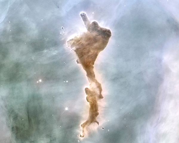
A Hubble view of a molecular cloud, roughly two light-years long, that has broken off of the Carina Nebula. [NASA/ESA, N. Smith (University of California, Berkeley)/The Hubble Heritage Team (STScI/AURA)]
Since we know that dense gas is required to form stars, it is natural to ask what relationship there is between the two. In fact, the Kennicutt–Schmidt (KS) relation tells us that there is a direct scaling between the mass of gas and the star formation rate (SFR). This relationship has allowed us to trace star formation throughout the history of the universe and understand how galaxies grow over cosmic time. But the authors of today’s paper asked a question that puts a slight twist on the KS relation: they wanted to know if such a relationship holds within individual molecular clouds.
Putting Clouds Under the Microscope
To answer this question, the authors used Spitzer and Herschel data for 12 well-studied star forming regions. Using the Herschel far-infrared data, they computed molecular hydrogen column density maps. With these measurements, they were able to compute the surface density of the gas in the star forming regions. With both near- and mid-infrared data from Spitzer the authors identified sources with a significant infrared excess and classified them into subclasses of young stellar objects (YSOs), also known as protostars. With these data, the authors measured the gas masses and number of stars within given density contours (corresponding to a physical area in the cloud). Figure 1 shows these values. From these, a gas surface density, a star formation surface density, and a free-fall timescale can be calculated. The authors assumed a stellar mass of 0.5 solar mass and a 0.5-Myr timescale to compute the SFR.
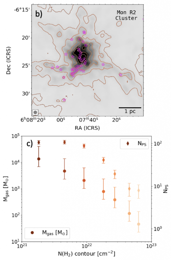
Figure 1: A strong correlation exists between the number of protostars and the gas column density. Top panel: Gas column density map of the Mon R2 molecular cloud. The brown contours indicate lines of constant surface density and the magenta stars are identified protostars. Bottom panel: Molecular gas mass (circles) and the number of protostars (diamonds) within each contour. [Pokhrel et al. 2021]
The Single Cloud Relation
With measured gas and SFR surface densities, the authors were ready to answer their main question. Figure 2 shows the comparison of these two quantities. As can be seen, the SFR surface density and the gas surface density scale strongly with each other. In fact, when normalizing by the free-fall timescale (right panel of Figure 2), the scatter in the relationship is decreased and the relationship becomes linear, as expected from theory.
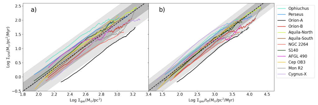
Figure 2: The gas and SFR surface densities are highly correlated. The above plot shows log of the SFR surface density as compared to the log of the gas surface density (left panel) and gas surface density divided by the free-fall time (right panel). The black line is the median best-fit relation and the dark and light gray shaded regions show one and two standard deviations from the fit respectively. [Pokhrel et al. 2021]
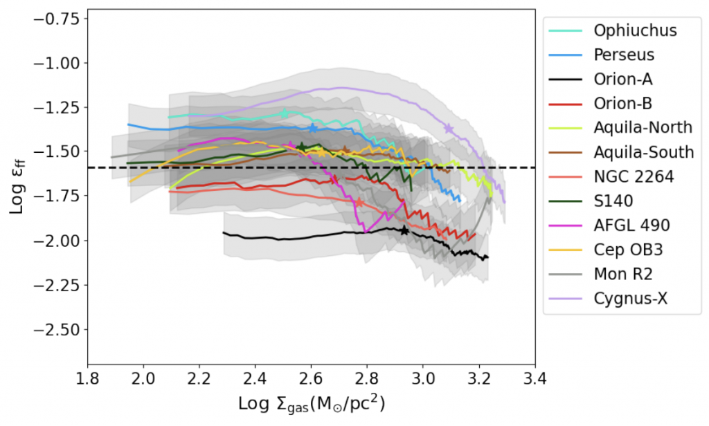
Figure 3: The gas surface density and free-fall efficiency are uncorrelated, suggesting the above relationship is real. The above plot shows log of free-fall efficiency as compared to the log of the gas surface density. The median log free-fall efficiency is shown by the black line. [Pokhrel et al. 2021]
In summary, the authors of today’s paper have shown that the KS relation that has been used for years in extragalactic studies has a local analog. This is particularly interesting as the various clouds in their sample have a wide range of physical properties. This correlation implies that star formation is regulated by processes on small scales, including stellar outflows or turbulence, rather than galaxy-scale effects such as supernovae and galactic properties. As we continue to study star formation in greater detail, the deeper meaning of this correlation may give us even deeper insights into how the stars we see every night were born.
Original astrobite edited by Suchitra Narayanan.
About the author, Jason Hinkle:
I am a graduate student at the University of Hawaii, Institute for Astronomy. My current research is on multi-wavelength photometric and spectroscopic follow-up of tidal disruption events. My research interests also include a number of topics related to AGN, including outflows, X-ray spectroscopy, and multi-wavelength variability. In addition to my love for astronomy, I enjoy hiking, sports, and musicals.