Editor’s note: Astrobites is a graduate-student-run organization that digests astrophysical literature for undergraduate students. As part of the partnership between the AAS and astrobites, we occasionally repost astrobites content here at AAS Nova. We hope you enjoy this post from astrobites; the original can be viewed at astrobites.org.
Title: Cosmic Velocity Field Reconstruction Using AI
Authors: Ziyong Wu et al.
First Author’s Institution: Sun Yat-Sen University, China
Status: Published in ApJ
Going with the (Hubble) Flow?
Hubble’s law is a beautifully simple statement: a galaxy caught in the Hubble flow, moving with the expansion of the universe, should be traveling away from us at a speed proportional to its distance. Unfortunately, however, this velocity–distance relation is too good to be true: due to the pesky influence of gravity, Hubble’s law is invalid in the vast majority of cases. In general, a galaxy’s net motion can be attributed to a combination of the Hubble flow, the galaxy’s motion within its galaxy cluster or group, and the motion of the cluster or group itself. We collectively refer to these deviations from the Hubble flow as “peculiar motions” or “peculiar velocities.”
While the presence of peculiar motions spoils the simplicity of Hubble’s law, these motions can be a blessing in disguise: since diversions from the Hubble flow are caused by gravitational interactions — and therefore by the presence of matter — peculiar motions serve as excellent probes for the physics of structure in the universe. Peculiar velocities have been used to map the cosmic web — the vast network of filaments connecting matter on the universe’s largest scales (explored further here, here, and here) — and are linked to the dynamics of galaxy clusters and the cosmic microwave background via the kinematic Sunyaev–Zel’dovich effect. Peculiar motions are also the root cause of redshift–space distortions, and thus one requires precision measurements of peculiar velocities in order to test cosmological models using the Alcock–Paczynski effect (see here and here for deeper explanations of this technique).
One caveat, though: measuring peculiar velocities is hard. To decouple peculiar motions from the Hubble flow observationally, we need a means of measuring distances that doesn’t require redshifts. To this end, a distance ladder or the Tully–Fisher and Faber–Jackson relations are viable methods, but each carry significant measurement uncertainty. Alternatively, we can take a theoretical approach, using perturbation theory to infer cosmic velocities from cosmic density data. However, any attempts to fully model the nonlinear growth of large-scale structure by hand quickly become prohibitively complex, necessitating a number of approximations and simplifications. How, then, can we accurately and efficiently compute peculiar velocities on cosmological scales? The authors of today’s paper may have found a solution in the field of machine learning: convolutional neural networks.
From Convolutions to Cosmology
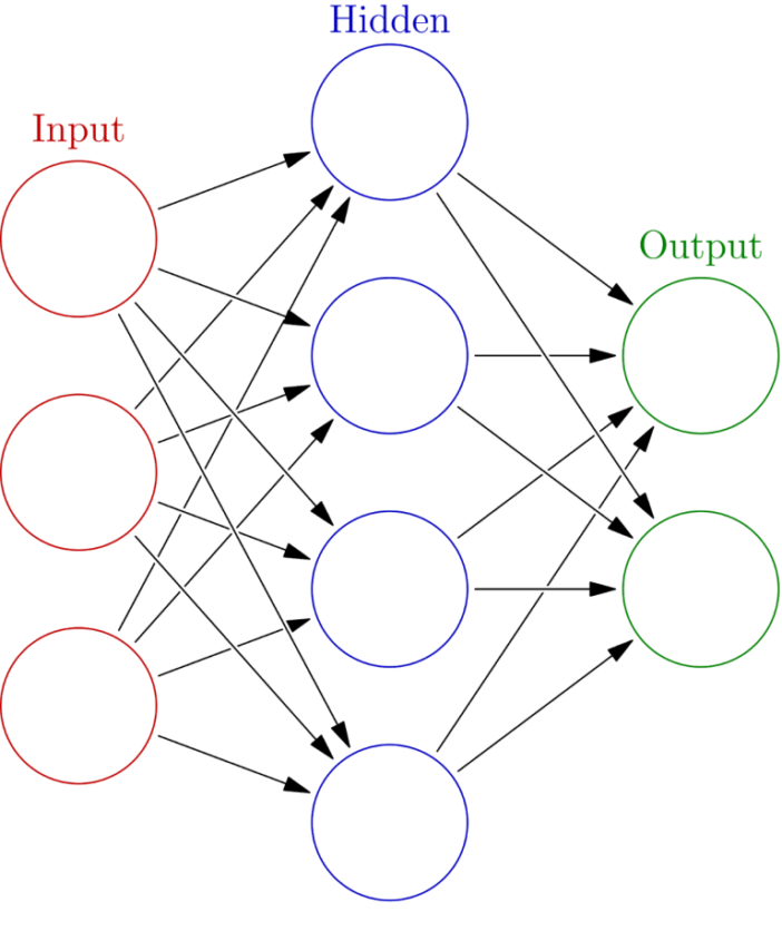
Artificial neural networks are, in essence, models with very many free parameters. As one trains the neural network by feeding it many input data sets and scoring its output against the expected results, the network adjusts its parameters, thus learning how best to map the given inputs to the desired outputs. Figure 1 shows a simple neural net with a fully connected three-layer “feed-forward” architecture; the data, in the form of an array of real numbers, is reprocessed as it’s transmitted from the “input layer” to a “hidden layer” and finally to the “output” layer. Each connection between layers bears a weight that dictates how a layer’s “neurons” should process their inputs — these weights are the free parameters in the neural network. Ultimately, neural nets produce models that are highly nonlinear, thus making them ideal for studying the complex dynamics of cosmic structure formation.

Figure 1: A schematic diagram of a fully connected three-layer feed-forward neural network, where each circle represents a neuron. Here, the data is fed into the input layer as an array, then transmitted to the hidden layer where it is mixed and reprocessed based on the weights of the connections leading into the hidden layer; the resulting values are sent to the output layer, where they are reprocessed one final time, ultimately producing a highly nonlinear model. [Glosser.ca]
To generate their training and testing data sets, the authors simulate the formation of large-scale structure up to the present day, retrieving both cosmic density and momentum maps; the density maps are used as inputs to the neural net, while the corresponding velocity maps — computed by dividing the momentum fields by the density fields — are used to evaluate the neural net’s output and to subsequently train, cross-validate, and test the resulting model.
Math vs. Machine
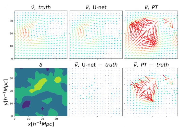
The authors assess the performance of their trained neural network by comparing its peculiar velocity predictions to those of linear perturbation theory. In nearly all cases, the neural net clearly outperforms the theoretical model. Perturbation theory performs well in regions of low density and velocity, occasionally yielding better predictions than the neural net. However, in regions of high density and velocity and in merger situations where two regions of opposing velocity collide with one another, perturbation theory fails completely, while the neural net still faithfully reconstructs the velocity field (see Figure 2). Over multiple testing data sets, the neural net is shown to be robust in all situations, while perturbation theory becomes practically useless in the presence of nonlinear dynamics.

Figure 2: Comparison of a simulated velocity field (upper left) with a field predicted by the neural network (upper middle) and by perturbation theory (upper right); the lower left shows the underlying density field, while the lower middle and lower right show the residuals for the neural net predictions and the perturbation theory predictions, respectively. In regions of high density and velocity and in regions of converging flow, perturbation theory breaks down. [Wu et al. 2021]
Original astrobite edited by Pratik Gandhi.
About the author, Ryan Golant:
I am a first-year astronomy Ph.D. student at Columbia University. My current research involves the use of particle-in-cell (PIC) simulations to study magnetic field growth in gamma-ray burst afterglows and closely related plasmas. I completed my undergraduate at Princeton University, and am originally from Northern Virginia. Outside of astronomy, I enjoy playing violin, studying art history, reading Wikipedia, and watching cat videos.
