
Ripples in Time: The Transient Nature of Mysterious M Stars
Editor’s Note: Astrobites is a graduate-student-run organization that digests astrophysical literature for undergraduate students. As part of the partnership between the AAS and astrobites, we occasionally repost astrobites content here at AAS Nova. We hope you enjoy this post from astrobites; the original can be viewed at astrobites.org.
Title: Transient Corotating Clumps Around Adolescent Low-Mass Stars from Four Years of TESS
Authors: Luke G. Bouma et al.
First Author’s Institution: California Institute of Technology
Status: Published in AJ
The flow of time gently pushes us all downstream, making the present past and the future present. So much of science, and even life, is trying to understand how time will change what we experience and observe. What remains the same? Is this something stable that we can rely on? What changes? Is this moment precious? Just a fleeting incident? And how can we tell the difference? These are hard questions, no matter the subject. Today’s authors are unfazed by the challenge and seek to understand what can be said about a mysterious group of M-dwarf stars that seem to be stable in their changing!
Complex Periodic Variables
The subjects of today’s study are complex periodic variables, a new name for objects previously called complex rotators and, before that, scallop-shell objects. While the name has changed, the type of object the name describes hasn’t. Complex periodic variables are all young (less than 200 million years old), rapidly spinning (rotation periods of less than two days), small M-dwarf stars. Only about 150 of them are known, and each has been associated with groups of other young stars, ranging from 2 to 200 million years of age.
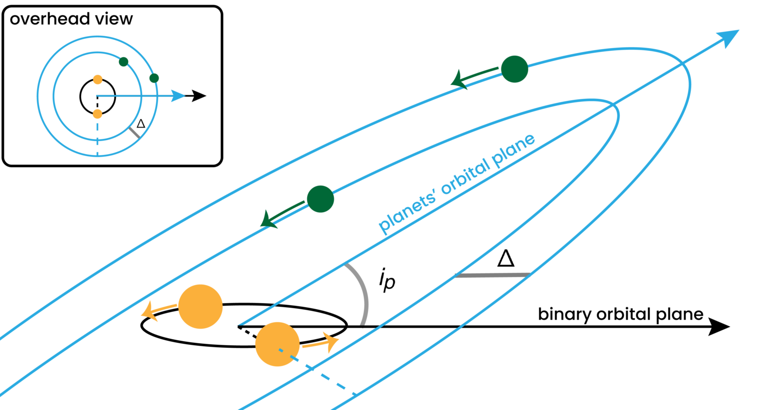
What makes complex periodic variables stand out from the crowd in their young groups are their light curves: the measure of their brightness over time. Young stars tend to have big, dark starspots on their surfaces that rotate into and out of view. Starspots normally produce a smooth repeating pattern in the light curve, varying at the spin rate of the star. However, complex periodic variables’ light curves show sudden, sharp repeating features rather than smooth ones. This can’t be caused by starspots alone, but like starspots, these repeating features are stable for weeks and seem to change with the star’s rotation. These sharp features are thought to be caused by either clumps of material orbiting at the right distance to be phased with the star and blocking starlight, or material in prominences formed off the surface of the star due to its magnetic field (Figure 1).
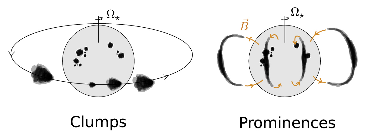
Figure 1: Two possible physical causes for the complex light curve shapes. The spotted star is seen with clumps of material orbiting around it (left), or with material trapped in the star’s magnetic field as prominences off the surface (right). [Adapted from Bouma et al. 2024]
What Remains the Same? What Changes?
To get a better handle on how stable these complex variations are, and to potentially find some more, the authors searched the two-minute-cadence data from the Transiting Exoplanet Survey Satellite (TESS) for objects with complex variability and found 50 of them. Many of the objects were previously known, but some were new, and the 50 objects served as a great data set for looking at the complex shapes of the light curves. Of the 50, a subset had observations at least two years apart. The authors show the difference in the repeating light curve shape for 27 of the objects in Figure 2.
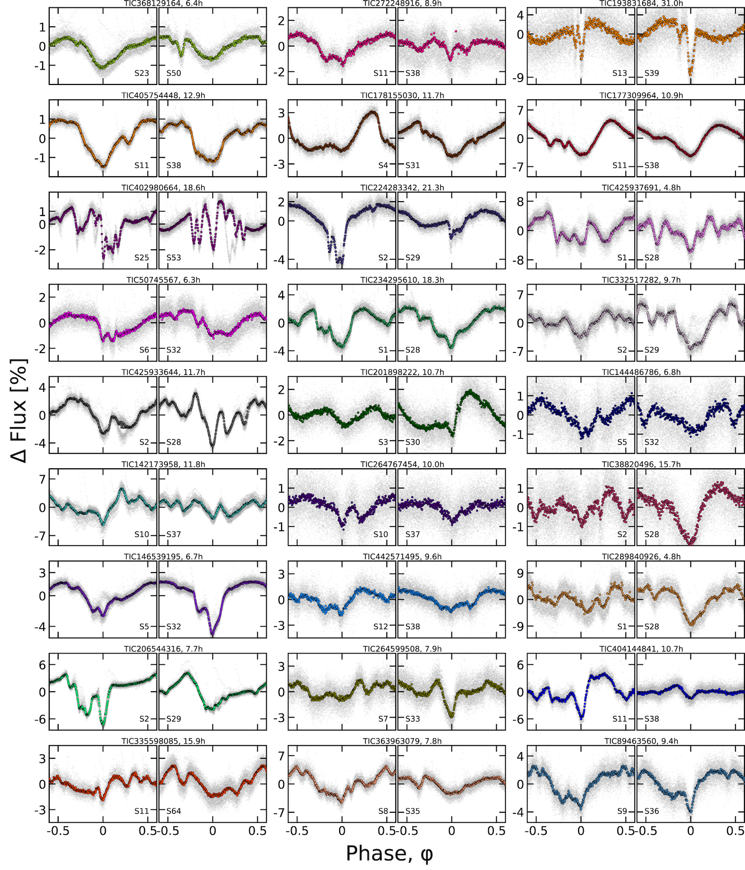
Figure 2: Twenty-seven complex periodic variables that have TESS observations separated by at least two years. For each object there are two panels, showing first the earlier and then the later observations. The x axis is the rotational phase, or when the star is in the repeating pattern, and the y axis is the percent change in brightness. Tag yourself, I’m TIC 264767454. [Bouma et al. 2024]
To examine that further, the authors did a deep dive on a particular star: LP 12-502. They broke up the light curve patterns even further; now, instead of looking at month-long TESS observation sectors, they look at a specific number of cycle repetitions for the object (Figure 3). This finer subdivision revealed that even after every 10–20 cycles of rotation there were subtle, and sometimes dramatic, changes in the shape of the light curve. Furthermore, they were able to point to noticeable flares occurring before some of the changes in the light curve, potentially pointing to a link between flares and changing light curve shape.
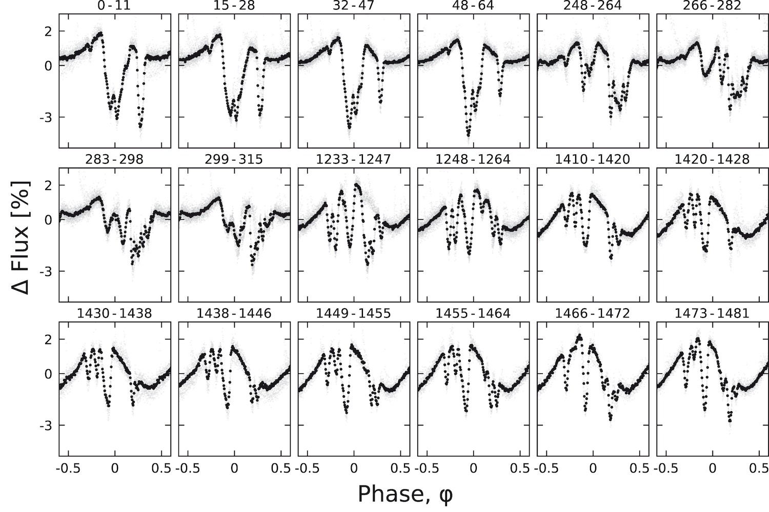
Figure 3: The light curves of the complex rotator LP 12-502 broken up over particular cycles of rotation (given in the title of each panel). Gaps in coverage are caused by TESS’s observation windows. The patterns of complexity shift and change subtly even over these short time frames. [Bouma et al. 2024]
The River of Time
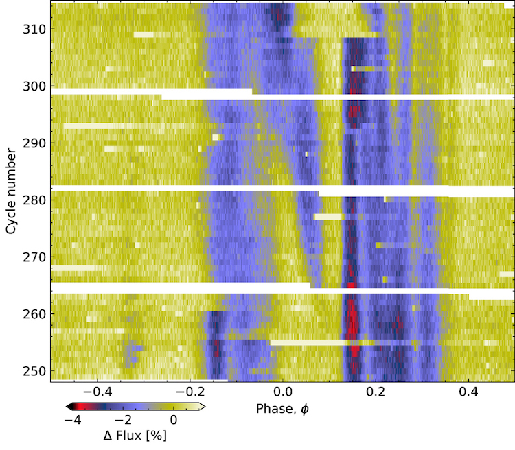
Figure 4: A river plot for the star LP 12-502, showing the change in brightness as a function of cycle on the y axis and rotational phase on the x axis. The light curve has been sliced into cycles of rotation and then converted into strips of color stacked on top of each other. [Adapted from Bouma et al. 2024]
I find these plots peaceful; I want to be sat in an inner tube, floating along their surface. Tough questions of change become easier when considered in comfort. The ripples of brightness ferry me down the lazy-flowing river of time, the gentle motion meandering my thoughts around the potential cause of these mysterious objects.
Original astrobite edited by Ivey Davis.
About the author, Mark Popinchalk:
I’m a postdoc at the American Museum of Natural History. I study the age of stars by measuring how quickly they rotate. I enjoy ultimate frisbee, baking bread, and all kinds of games. My favorite color is sky-blue-pink.


