Editor’s note: AAS Nova is on vacation until 2 November. Normal posting will resume at that time; in the meantime, we’ll be taking this opportunity to look at a few interesting AAS journal articles that have recently been in the news or drawn attention.
The question of what happens after two neutron stars collide is still an open one — thrown into the spotlight in recent years with the detection of a gravitational-wave signal coincident with electromagnetic radiation from the neutron-star collision GW170817. Scientists are actively working to improve models of this process, and the latest comes from a team led by Philipp Mösta (University of Amsterdam). The authors’ 3D models show what might happen to a post-collision remnant — a hypermassive neutron star — as it evolves over time, gaining magnetic field strength and launching dramatic, relativistic jets and neutron-rich winds. The simulations show how a burst of gamma rays can be produced, as well as heavy elements like gold, all nicely matching observations of the 2017 merger.
Check out the video below to watch the authors’ simulated remnant (and its magnetic field lines) evolve for yourself.
Editor’s note: AAS Nova is on vacation until 2 November. Normal posting will resume at that time; in the meantime, we’ll be taking this opportunity to look at a few interesting AAS journal articles that have recently been in the news or drawn attention.
Scientists have discovered a monster in the early universe, and it’s challenging our understanding of how black holes grow. A recent study led by Jinyi Yang (Steward Observatory, University of Arizona) details the detection of a massive quasar — the bright, accreting supermassive black hole at the center of an active galaxy — at a redshift of z = 7.515, a distance corresponding to a time just 700 million years after the Big Bang. The quasar was detected using three observatories on Maunakea in Hawai’i, and it was given the name Pōniuā’ena. This monster is the second-most distant quasar known — and, weighing in at roughly 1.5 billion solar masses, it’s nearly twice the size of the most distant quasar we’ve detected.
We think that the first stars, galaxies, and black holes began to form during the Epoch of Reionization, roughly 400 million years after the Big Bang. Pōniuā’ena’s existence therefore poses a puzzle: how could a black hole possibly grow to such an enormous size in just 300 million years?
Check out the video below for an overview of the discovery from Keck Observatory, as well as some insight into the quasar’s name.
Editor’s note: AAS Nova is on vacation until 2 November. Normal posting will resume at that time; in the meantime, we’ll be taking this opportunity to look at a few interesting AAS journal articles that have recently been in the news or drawn attention.
What’s your computer doing when you’re not using it? It could be discovering hidden, record-breaking pulsars, like in the case of PSR J1653−0158, recently found via the Einstein@Home project.
Einstein@Home is a distributed computing project that uses idle computer hours from volunteers to speed up computationally expensive searches for signatures of pulsing neutron stars — pulsars — in large datasets from observatories like the LIGO gravitational-wave detectors, large radio telescopes, and the Fermi Gamma-ray Space Telescope. The donated hours can shorten hunts from what would normally take centuries on a single computer to just a couple weeks.
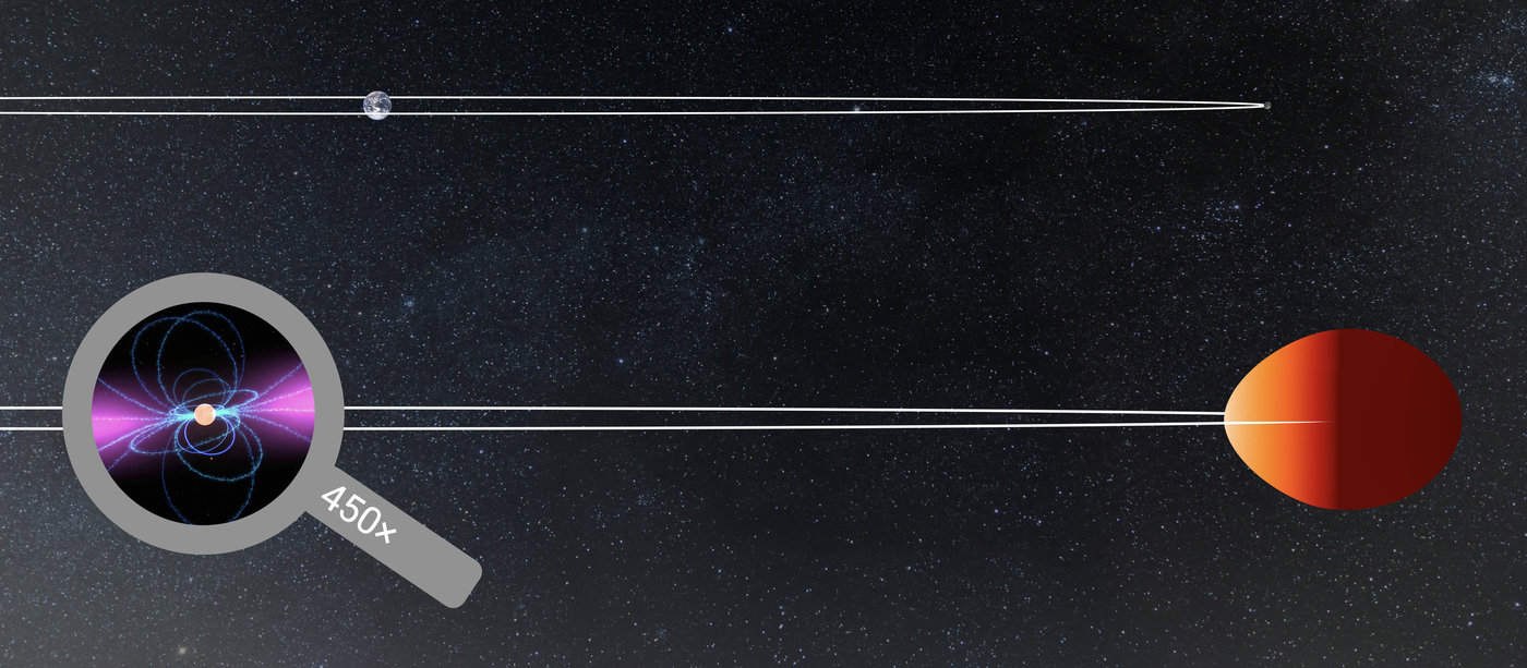
In a new study led by Lars Nieder (Albert Einstein Institute, Germany), scientists announced the Einstein@Home project’s latest discovery: a gamma-ray-bright but radio-invisible pulsar in an orbit with an extremely low-mass star. Such a system is called a “black widow pulsar” — because the pulsar is destroying its companion! — and this one sets a number of records for these systems: it has the fastest orbital period (75 minutes), and the pulsar is unusually massive and has one of the fastest spins and weakest surface magnetic fields of known pulsars.
You can read more about the discovery, and about Einstein@Home, in the original article and the press release below.
Illustration of the binary star system with the pulsar J1653-0158 (bottom) in comparison to the Earth-Moon system (top). The pulsar is magnified by 450x, but all other sizes and distances are to scale. [Knispel/Clark/Max Planck Institute for Gravitational Physics/NASA]
Editor’s note: AAS Nova is on vacation until 2 November. Normal posting will resume at that time; in the meantime, we’ll be taking this opportunity to look at a few interesting AAS journal articles that have recently been in the news or drawn attention.
Can life survive the death of its star? Planets orbiting white dwarfs present a unique opportunity to characterize rocky worlds in an attempt to answer this question. Scientists Lisa Kaltenegger and Ryan MacDonald (Cornell University) and collaborators have now shown that the upcoming James Webb Space Telescope (JWST) will be capable of establishing the atmospheric composition of planets transiting white dwarfs in their habitable zones. JWST could detect potential biosignatures in the atmospheres of these planets in as few as 25 transits — which, given the short transit duration for habitable-zone planets around white dwarfs, amounts to a small investment of observing time. For this reason, the authors argue that white dwarfs present a valuable target for future JWST observations. Check out the video below, in which Kaltenegger and MacDonald make their case for why we should explore white dwarfs in the search for life.
In August of 2015, AAS Nova launched as a new service provided by the AAS journals. Today, five years later, we’re officially celebrating the milestone of the 1,000th Highlight post published on the site.
Beyond functioning as a news service, AAS Nova acts as an archive of astronomy research — which provides us with an interesting opportunity to explore how our understanding of the universe has developed.
Today we’re taking a moment to look back at a tiny sample of the new discoveries and ideas published across different corridors in the AAS journals and highlighted on AAS Nova over the past half-decade.
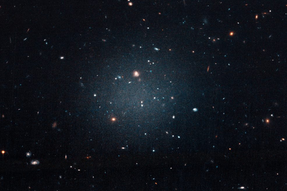
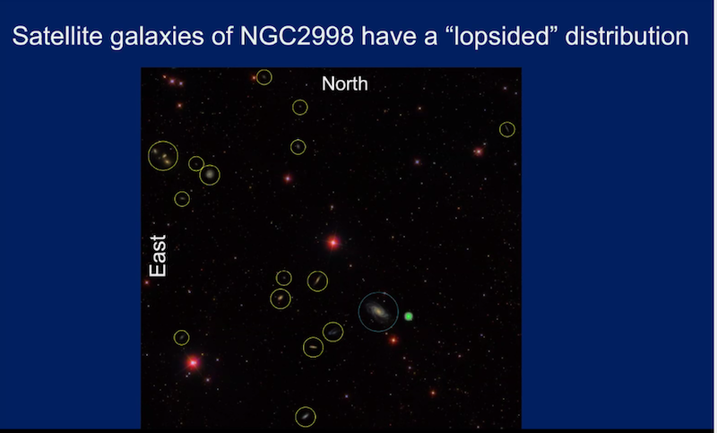
The faint object in the center of this image is NGC 1052-DF2, an ultra-diffuse galaxy at the center of a scientific debate about dark matter. [NASA/ESA/P. van Dokkum (Yale University)]
We’ve also continued to make progress toward resolving a number of long-standing debates, such as the question of why we don’t see as many small satellite galaxies as predicted (the “missing satellite problem”), or why our two methods of measuring the Hubble constant — a number that describes the rate of expansion of the universe — come up with different results.
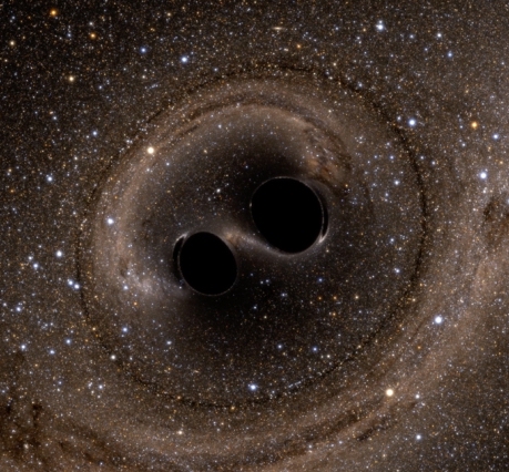
Simulated image of two merging black holes, viewed face-on. LIGO announced the detection of ten of these events from its first two observing runs. [SXS Lensing]
High-Energy Phenomena and Fundamental Physics
One of the biggest headlines in the past five years was the first detection of gravitational waves from a merging pair of black holes. Since this discovery, the Laser Interferometer Gravitational-wave Observatory (LIGO) and its European counterpart, Virgo, have detected more than a dozen mergers of compact objects, and observatories across the world have searched for — and found! — electromagnetic counterparts to these collisions. Theoretical models of compact binary formation and evolution have also advanced in leaps and bounds as we’ve learned more.
Continuing the theme of “cool new observations of black holes”, the Event Horizon Telescope presented its view of M87 last year, opening a window onto what’s happening in the innermost regions around supermassive black holes. And we’ve amassed dozens of observations of black holes tearing apart passing stars in tidal disruption events, improving our models of this destruction in the process.
But outbursts from black holes aren’t the only transient phenomena flashing through our skies. The past few years have dramatically advanced our understanding of fast radio bursts, sudden, brief bursts of radio emission that originate from outside our galaxy. We now suspect these flashes might be related to high-energy phenomena, like the birth or evolution of distant magnetars.
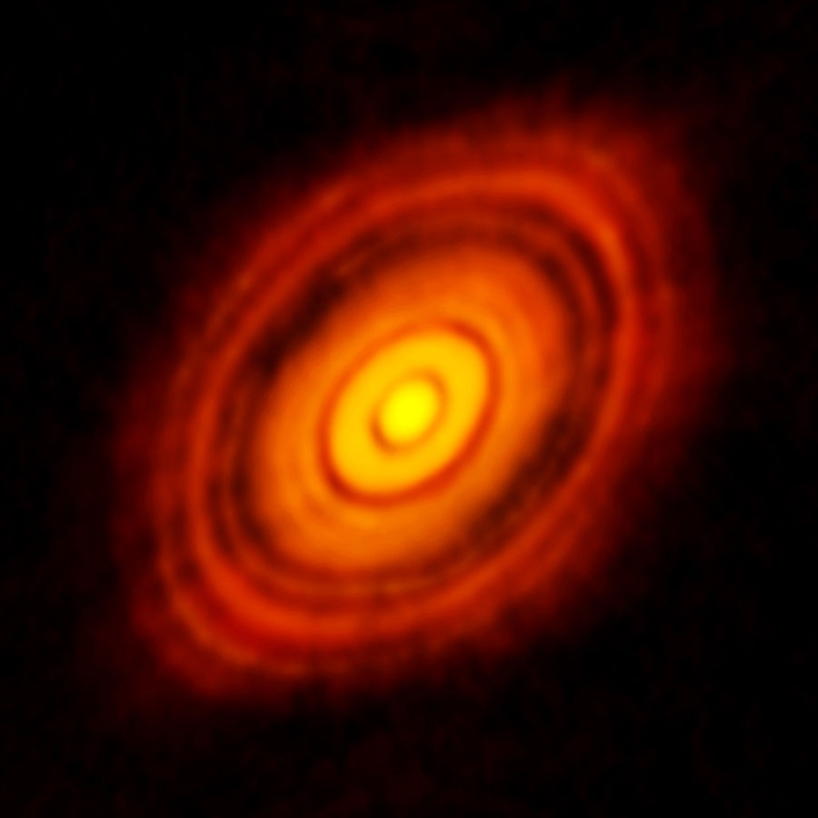
This ALMA image of the protoplanetary disk surrounding the star HL Tauri reveals the detailed substructure of the disk, including gaps that may have been cleared by planets. [ALMA (ESO/NAOJ/NRAO)]
Interstellar Matter and the Local Universe
One of the biggest new players in the study of gas and dust in the local universe is the Atacama Large Millimeter/submillimeter Array (ALMA), which announced new results from its first long-baseline, high-resolution campaign around the time that AAS Nova first launched. Since then, ALMA has continued to produce spectacular observations — the array is mentioned in 82 of the 1,000 Highlights currently posted on AAS Nova, indicating the transformative nature of its observations.
As we peer deeper into interstellar clouds, we’ve also discovered a number of new molecules in the gas and dust of the universe, broadening our interstellar census and helping us to better understand our origins. Additionally, we’ve made significant advances in understanding the structure of magnetic fields in dense interstellar clouds and unraveling the role that they play in star formation.
Artist’s illustration of the Breakthrough Starshot Initiative, a plan to send a fleet of tiny spacecraft to Alpha Centauri. [Breakthrough Initiatives]
Laboratory Astrophysics, Instrumentation, and Software
While the most headline-grabbing astronomy is often major detections and observations, more attention has started to come to the important underlying work of exploring astrophysical phenomena in the lab — from the construction of white dwarf photospheres to the formation of dust grains under conditions mimicking the cold vacuum of space — and developing new and increasingly advanced instrumentation and software.
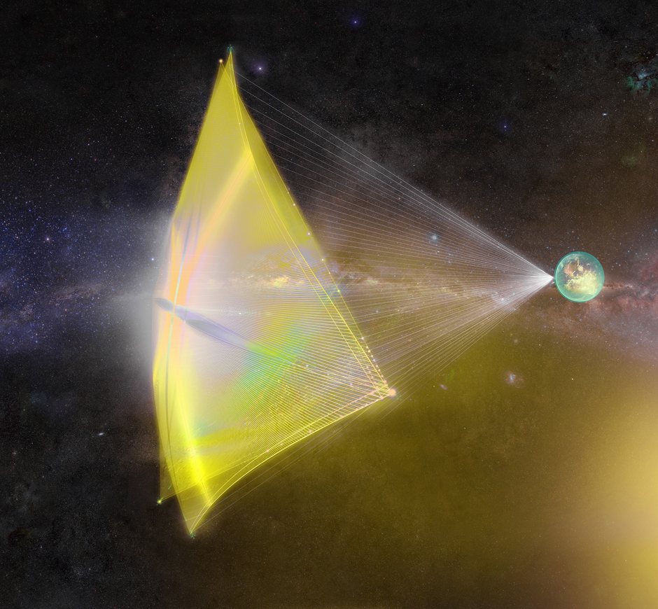
Human-made objects in space continue to both inspire and trigger debate. Recent developments include the Breakthrough Starshot Initiative to send a fleet of centimeter-sized spacecraft to the nearest star system, as well as the influx of satellites in low-Earth orbit and the impact this has on astronomy.
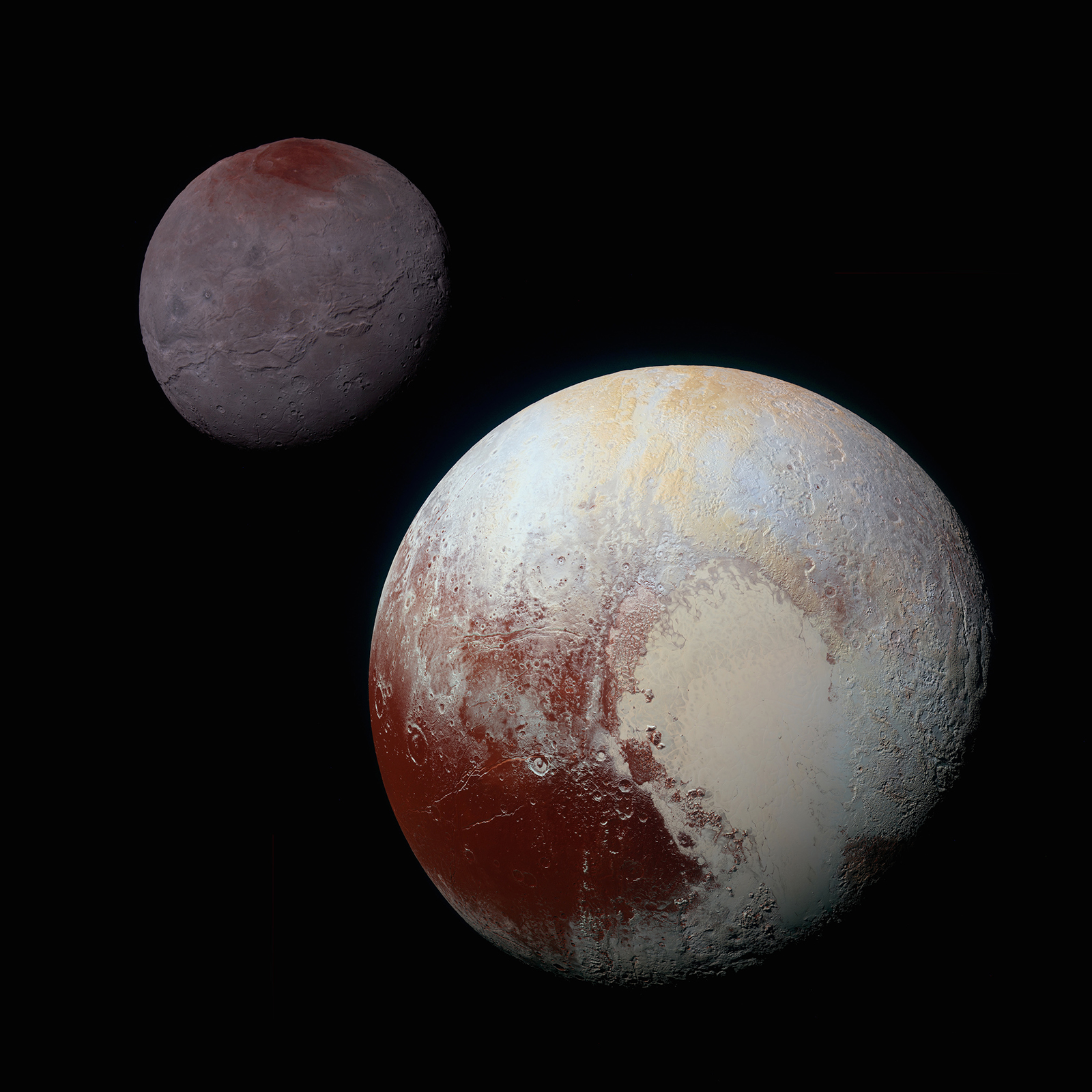
This composite image with enhanced colors shows New Horizons observations of Pluto (foreground) and Charon (background). [NASA/JHUAPL/SwRI]
On the small-body front, the New Horizons spacecraft flew by Pluto just before AAS Nova launched, and it then followed up with an up-close look at asteroid MU 69. Multiple interstellar asteroids have recently been observed as they pass through our solar system, and missions are underway to actually land on asteroids and return samples to Earth.
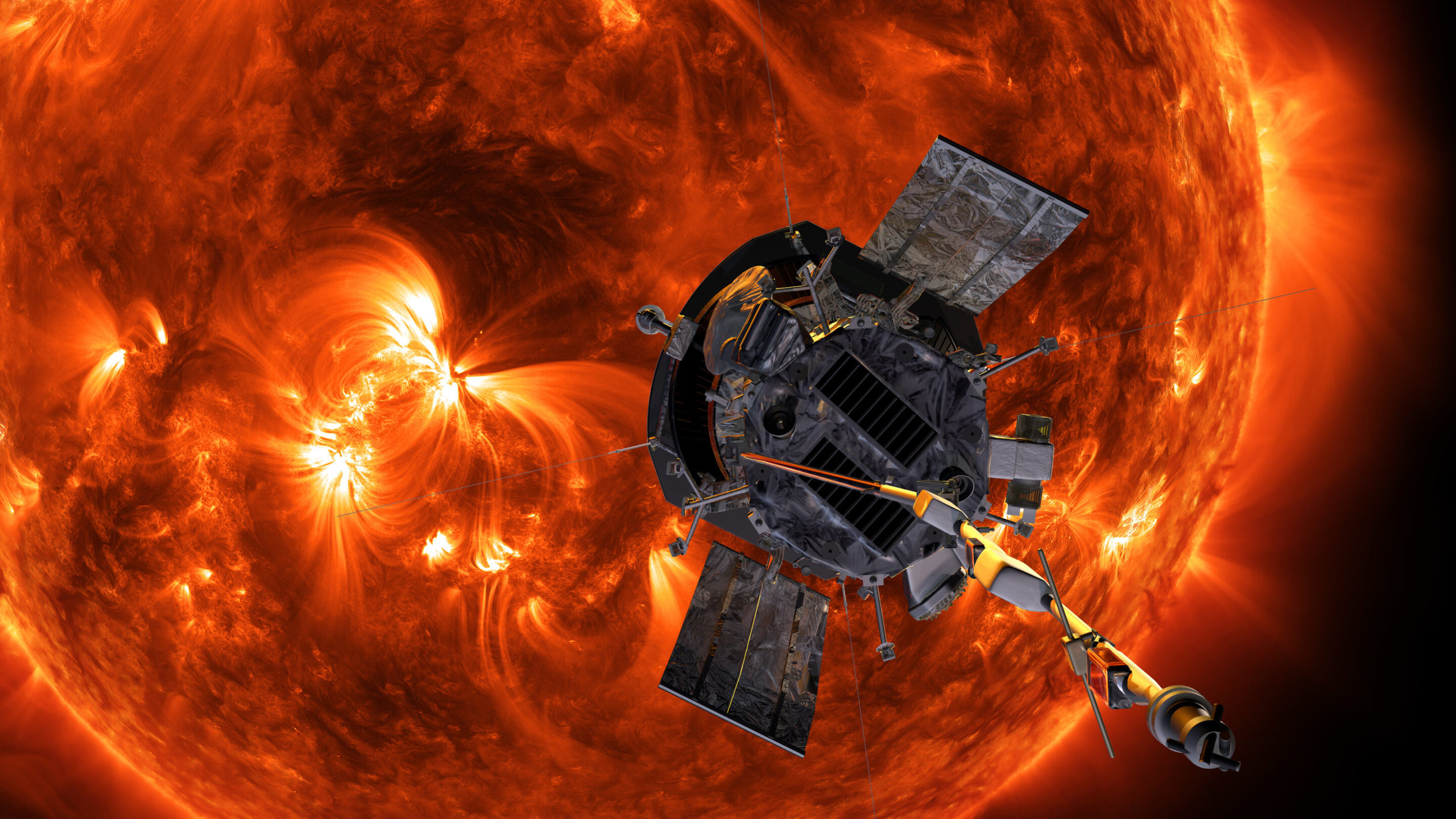
Artist’s illustration of the Parker Solar Probe. A special ApJS issue features around 50 articles detailing early results from this mission. [NASA/Johns Hopkins APL/Steve Gribben]
The Sun and the Heliosphere
In solar physics, we’ve continued to make steady progress toward solving major mysteries of our Sun, like how particles are accelerated in energetic solar flares, and why the outer solar corona is so much hotter than the layers of the Sun’s atmosphere that lie below it (the so-called coronal heating problem). We’re also gaining a better understanding of our broader solar system as the Voyager satellites and IBEX explore the heliosphere.
In addition to the large assortment of Sun-observing telescopes already on the job, we’re still finding new ways to explore our nearest star — from hard X-ray images to balloon-borne ultraviolet observations. An especially unique view is now coming from the Parker Solar Probe, a spacecraft that recently arrived at the Sun and is already producing results. This probe will continue to plunge ever closer to the Sun’s surface over the next five years.
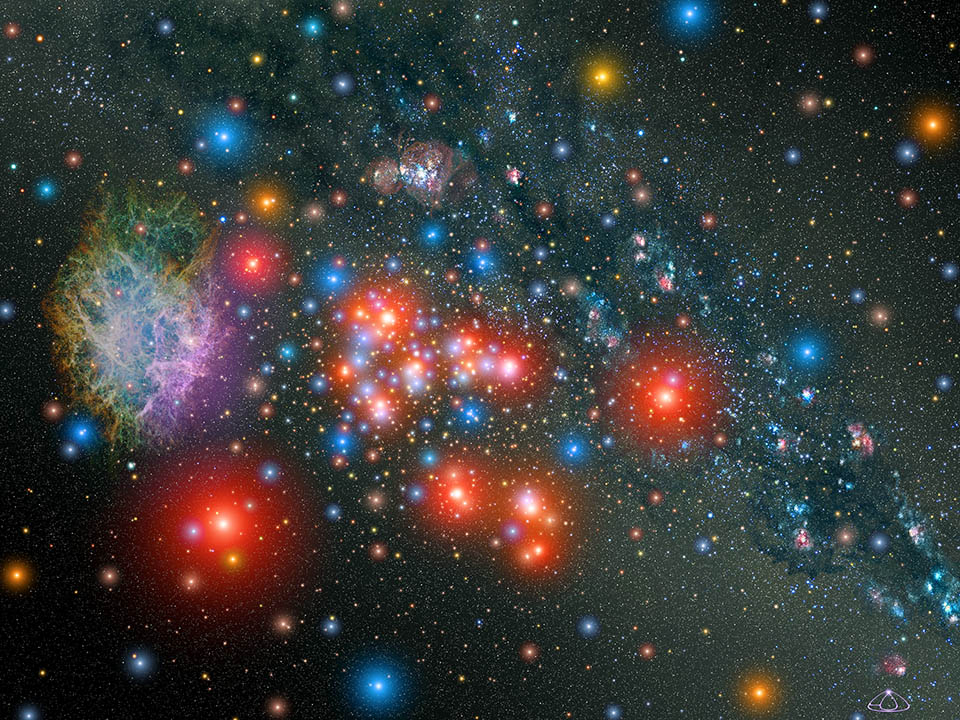
Artist’s illustration of one of the most massive star clusters within the Milky Way. The center of the cluster contains 14 red supergiant stars. [NASA, ESA and A. Schaller (for STScI)]
A huge astronomical milestone was achieved with Gaia’s first and second data releases, which map the positions, parallaxes, and proper motions for more than a billion stars and have enabled a wealth of studies of our surrounding galaxy.
There are, of course, many more astronomical successes from the past half-decade than could be summarized in a short post here. Even so, this look back on the past five years of astronomy provides a clear sense of the remarkable advances we’ve made in a relatively short time.
It should be noted that our advances don’t negate the challenges that our field still faces — we have plenty of problems to address, like racial diversity, equity, and inclusion in astronomy. Nonetheless, as we look both inward and outward, we’re making steady progress toward understanding the universe around us and our role in it.
At AAS Nova, we’ve loved reporting on all that’s happened in astronomy over the past five years. We’re excited to see what the next five bring!
Editor’s Note: This week we’re at the 236th AAS Meeting, being conducted virtually for the first time! Along with a team of authors from Astrobites, we will be writing updates on selected events at the meeting and posting each day. Follow along here or at astrobites.com. The usual posting schedule for AAS Nova will resume the week of June 8th.
Solar Physics Division (SPD) Hale Prize Lecture: From Jets to Superflares: Extraordinary Activity of Magnetized Plasmas in the Universe (by Abby Waggoner)
The last day of AAS 236 started off with the Solar Physics Division Hale Prize Lecture by Kazunari Shibata from Kyoto University. Dr. Shibata was awarded the Hale prize for his years of research on magnetized solar and astrophysical plasma and the discovery of solar jets. Dr. Shibata is the first scientist from Japan to receive the Hale prize, which is the most prestigious award in solar physics.
Dr. Shibata didn’t always study solar physics. During his graduate studies (1973–1977) he sought to solve the “biggest puzzle in astrophysics”: the jets produced by active galactic nuclei (AGN). A series of jets were discovered in the 1960s, but the physics behind them was unknown at the time. AGN are difficult to observe directly, as they are billions of light-years away from Earth, so Dr. Shibata approached the problem from the theory side by studying magnetohydrodynamic (MHD) plasma. When the first protostellar jets were discovered, Dr. Shibata noticed that the morphologies of protostellar jets and AGN jets were similar, thus indicating that the jets were likely driven by the same physics.
At this point in time, scientists understood that jets in AGN originated from the transfer of kinetic energy produced by accretion, but the process by which the gravitational energy is converted to kinetic energy was still unknown. Dr. Shibata believed that the magnetic fields on the Sun were the key to understanding this, and he was right! He noticed that the spinning jets on the Sun could be related to the twist of a magnetic field.
This relation was confirmed when simultaneous observations in H-alpha and X-ray light were done on a single flare. Solar flare production by magnetic reconnection became known as the standard model. Dr. Shibata was able to connect the standard model to jets produced by AGN. Convection and rotation in the Sun (stellar dynamo) allow for the magnetic reconnection of magnetic field lines on the Sun, while accretion and rotation of the accretion disk around a black hole enables magnetic reconnection in AGN.
In the 1960s, the standard flare model was developed. Below the prominence, we have antiparallel lines that release magnetic energy. pic.twitter.com/yx4TbkrM1T
Dr. Shibata concluded his talk by discussing statistics done on the frequency of solar flares and the significance of “super flares.” He found that a super flare (energy range > 1033 erg, which is a lot of energy) could be produced by the Sun once every ~10,000 years. While we’ve never observed a super flare (luckily), he commented that a super flare could possibly be related to the origin and evolution to life on Earth.
(Conclusions continued) -"Extreme activity (such as superflares) on the Sun may have been related to the origin and evolution of life on Earth, whereas it would be extremely dangerous for our civilization in the future."
Press Conference: Mysteries of the Milky Way (by Haley Wahl)
Today’s first press conference follows on the heels of yesterday’s conference on the galactic center, and focuses on the broader picture of things.
The first speaker today was Dhanesh Krishnarao, a graduate student at the University of Wisconsin, Madison, speaking on the Fermi bubbles, which are massive lobes that expand out from the center of the galaxy. It’s known that these bubbles absorb light, but Krishnarao and his team discovered that they actually emit light too, and this was all seen by the Wisconsin H-Alpha Mapper, or WHAM! By measuring the optical emission and combining it with the UV absorption data, they were able to conclude that the Fermi bubbles have a high density and pressure. Press release
First discovery of optical light coming from Fermi Bubbles, paper on the ArXiv yesterday (arXiv:2006.00010)! Here's an artist's impression of the bubbles #AAS236pic.twitter.com/JOZVEwHEe9
The next speaker was Dr. Smita Mathur from Ohio State University to discuss a new discovery in the circumgalactic medium of the Milky Way. Before this work, the circumgalactic medium was thought to be mostly warm at temperatures around one million Kelvin. However, Mathur’s team discovered a hot component that’s around ten times as hot. No theory has ever predicted this!
How ubiquitous is that hot component of the circumgalactic medium? Dr.Anjali Gupta from Columbus State Community College, the third speaker of the press conference, explained! Using the Suzaku and Chandra telescopes, the team, led mostly by undergrad student Joshua Kingsbury, found the component in three out of the four sightlines they looked at. This hints at the fact that this hot component of the circumgalactic medium could be present in every direction, but more observations are needed. How can this hot component be explained? It’s possible that it could be related to feedback, from active galactic nuclei and/or from stars (star formation and supernovae)! Press release
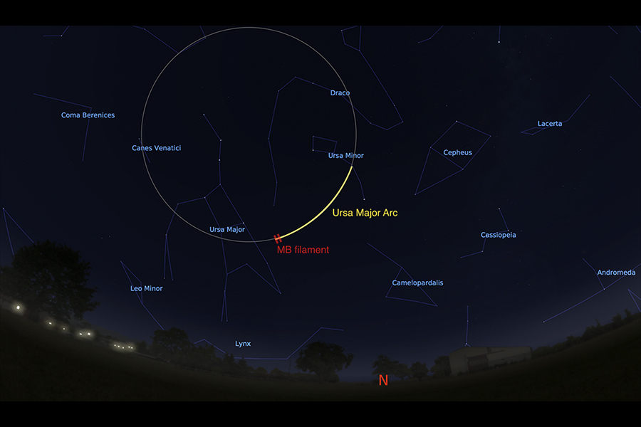
The location of the Ursa Major Arc relative to the Big Dipper. [Stellarium.org/A]
The last speaker of the press conference was Dr. Robert Benjamin from the University of Wisconsin, Whitewater, who spoke on a surprising result in a familiar sight in the nighttime sky. Benjamin and his team discovered a thin UV arc shock front whose length in the sky is 30° — that’s 60x the apparent size of the full Moon! If the arc were extended, it would make an enormous circle on the sky with a radius that’s also 30° in size. They believe the arc to be about ~100,000 years old and >600 light-years away and possibly caused by a supernova; if this is the case, it would be the largest supernova remnant in the sky. Press release
Plenary Lecture: Our Dynamic Solar Neighborhood (by Luna Zagorac)
Jacqueline Faherty (American Museum of Natural History) studies our solar neighborhood (20–500 pc from the Sun) because it lets us investigate faint sources in more detail, including brown dwarfs. One important question we can begin to answer in the solar neighborhood is where the high-mass limit of planet formation ends and the low-mass limit of star formation begins. To illustrate what the stellar neighborhood looks like, Dr. Faherty took us on a virtual flight using the OpenSpace software, illustrating the advancement in mapping and astrometry from the Hipparcos data set to Gaia DR2, which mapped more than 1.3 billion sources. Gaia is an optical survey and, as such, is not very sensitive to faint, cold sources like brown dwarfs. When Gaia data was combined with ground-based measurements, however, 5,400 sources were extracted from the sample of Gaia objects within 20 parsecs of the Sun. These sources could then be arranged on a color-magnitude diagram (known as an HR diagram), with brown dwarfs clustering in the lower-left part of the diagram.
Here's these satellites plotted on a color magnitude diagram (an HR diagram)! White dwarfs in the lower left corner. pic.twitter.com/3snO7H8JNn
The scatter and differentiations in the diagram give insight into atmospheric characteristics of the colder objects represented. The coldest objects at the end of the spectral sequence, named Y dwarfs, are difficult to find because they’re not very luminous. Their temperatures are around 400 K, and their masses are estimated at ~20 Jupiter masses. These are the very markers of the transition between the bottom of the star formation process to the top of the planet formation process. The best way of identifying these objects has been through citizen science projects — the human eyes are the best recourse we have for identifying brown dwarfs!
Adding the discoveries from the Backyard Worlds citizen science project to the Gaia DR2 20 parsec sample will allow further constraining of brown dwarfs’ mass function. Citizen scientists are also helping to identify co-moving companions to stars, since their mass and separation distribution reveals more information about their formation. This is important because age can determine the mass of the object: “In determining co-moving structures, we can measure their ages and we can use those to do a deeper dive to systems within them,” noted Dr. Faherty. This project is being led by her postdoc, Dr. Daniella Bardalez Gagliuffi.
Furthermore, there are objects in the Tucana-Horologium Association that are in systems where a companion has been discovered right on the mass boundary between planet and brown dwarf formation. These companions resemble Jupiter and have thick clouds, and Dr. Faherty wants to study how their light is changing. To find more of these systems, her former student Dr. Eileen Gonzales is developing BREWSTER, a retrieval code optimized for brown dwarfs, but adaptable to planets as well.
"These companions are at a temperature that's kind of crazy." Here's an example. They look a lot like Jupiter and have thick clouds. We want to look at how their light is changing. pic.twitter.com/9Oz4W4pLwj
These data sets have allowed us to better visualize low-luminosity object distributions in the sky, and Dr. Faherty hopes this can be turned into planetarium presentations. She concludes that the multi-dimensional nature of stellar catalogs is highly complemented by visualization tools and that the James Webb Space Telescope will be critical in further characterizing these low-luminosity objects.
OSTP Town Hall with White House Science Advisor Kelvin Droegemeier (by Tarini Konchady)
Note: In the recording of this session, Dr. Droegemeier’s audio for the Q&A was lost. This writeup covers everything that was said before the Q&A.
The main speaker at the Office of Science and Technology Policy (OSTP) town hall was Director Kelvin Droegemeier. Droegemeier’s scientific background is in meteorology; in 1985 he joined the University of Oklahoma as an assistant professor and has remained at that institution to this day (he has taken a leave of absence to serve as OSTP director). Droegemeier has a long career in federal policy as well, notably serving on the National Science Board from 2004 to 2016. Aside from being OSTP director, Droegemeier is also the Acting Director of the National Science Foundation. He will stay in this role till the Senate confirms the president’s nominee — Sethuraman Panchanathan — for the job.
The Office of Science and Technology Policy (OSTP) Town Hall happening now! Today's speaker is Dr. Kelvin Droegemeier, OSTP Director and Acting NSF Director.#aas236
Droegemeier emphasized that his experience as a college professor has informed his work in the federal government. He spoke about two particular OSTP efforts relevant to the AAS: one, helping colleges and universities with “reopening and reinvigorating” after the pandemic, and two, enabling research that would benefit the country.
To the first point, Droegemeier listed various meetings that have been happening between university leadership and federal bodies (including the Vice President and the National Science and Technology Council) as well as guidance issued by the government. He used these examples to emphasize that the government is apparently willing to give institutions leeway if it will allow smoother operations during the pandemic.
Droegemeier briefly switched gears to share the most recent status of astronomical facilities per James Ulvestad, Chief Officer for Research Facilities. Nothing differed significantly from the update given at the NSF town hall yesterday, though Droegemeier mentioned that the parking lot of the National Solar Observatory’s Boulder facility had been used for COVID-19 drive-through testing till recently. Construction on the dome and telescope mount of the Vera Rubin Observatory are unlikely to resume until September or October.
Droegemeier then pivoted back to OSTP business with an update on the Joint Committee of Research and Enterprise (JCORE), which was formed a little over a year ago. The four areas JCORE focuses on are research security, research integrity and robustness, research administrative workload, and safe and inclusive research environments. Droegemeier emphasized that the committee was continuing to work through the pandemic, especially the research security subcommittee.
In the same vein, Droegemeier spoke about how he had been going around the country to talk to faculty, students, and researchers about research security prior to the pandemic. Lisa Nichols, the OSTP Assistant Director of Academic Engagement, was also part of this effort.
Around this time of year, the OSTP issues an R&D guidance memo to federal agencies, setting priorities for the next fiscal year. The memo is purely guidance and does not contain any funding. Two of the key topics of last year’s memo was American security and “industries of the future” — technologies like artificial intelligence and 5G connectivity.
National High Performance Computing User Facilities Town Hall (by Sanjana Curtis)
The National High Performance Computing (HPC) User Facilities town hall was kicked off by Dr. Richard Gerber (NERSC) who introduced the goals of the town hall: inform the community about HPC and new directions in HPC, discuss opportunities for using HPC to advance astronomy research, communicate what is available at National HPC centers, and gather feedback from the community about their questions, needs and challenges. He also introduced the other presenters from major HPC facilities around the US: Niall Gaffney (TACC, UT Austin), Michael Norman (SDSC, UCSD), Jini Ramprakash (ALCF, Argonne National Lab), Bronson Messer (OLCF, Oak Ridge National Lab), and Bill Kramer (NCSA/Blue Waters, UIUC).
Dr. Gerber defined HPC as computing and analysis for science at a scale beyond what is available locally, for example, at a university. HPC centers have unique resources, including supercomputers, big data systems, wide-area networking for moving data quickly, and ecosystems that are designed for science (for, e.g.: optimized software for simulations, analytics, artificial intelligence and deep learning). These centers also offer lots of support and expertise, since they are staffed by people who are experts in HPC, many of whom have a science background. This helps bridge the gap between the domains of science and computing.
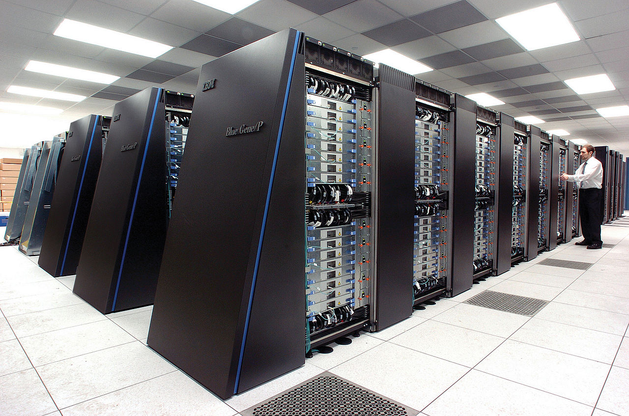
The IBM Blue Gene/P supercomputer “Intrepid”. [Argonne National Laboratory]
The traditional picture of a supercomputer is a system consisting of hundreds of thousands of the world’s fastest processors, coupled together by very high speed custom networks. Typically, they have a large scratch disk (~petabytes) optimized for reading and writing large chunks of data. These machines were originally designed to have all their compute nodes tightly coupled, where each node needs to know what the other nodes are doing, mainly to solve partial differential equations using linear algebra — they are really good at matrix multiplications! Users interact with supercomputers via SSH and command line, and submit their jobs to a scheduler or queue system for execution.
However, the HPC landscape is now changing, and rather abruptly! Single-thread processor performance growth that used to be exponential (Moore’s law-like) has stalled. Instead, we have to rely on parallelism and accelerators for increase in performance. Demand for data analysis is expanding, both from experimental and observational facilities, and large collaborative teams have become the norm. We are also witnessing the rise of artificial intelligence (AI), machine learning, and other emerging technologies with new needs.
So what’s next for HPC? According to Dr. Gerber, HPC will continue to advance the limits of computation and analysis. We will see data-intensive science and simulation science merging together, and large scale analysis of experimental and observational data moving to HPC. Since AI and deep learning are here to stay, HPC centers will have to accommodate this demand. Finally, supporting large collaborations will require enabling tools, such as tools for user authentication and data management.
Dr. Niall Gaffney (TACC) was up next, speaking about Astronomy and Advanced Computing in the 21st Century. He started out by mentioning the three pillars of modern computational science: simulation, analytics and machine learning/AI. Astronomy and computing are old friends and there exists a long list of very impressive simulations, such as the Renaissance Simulation, the SciDAC Terascale Supernova Initiative, black hole merger simulations for LIGO, and more! These large simulations are what people typically associate with supercomputing centers. However, there was a shift in this paradigm whenSDSS came online and showed astronomy the power of large-scale data and compute resources. The notion of a data center where you could go to run your analysis, without having to download huge quantities of data, was a big change. Now, there is an explosion of AI and machine learning methods, required by facilities like the Vera Rubin Observatory that will generate large amounts of data at very high rates. Astronomy has always been at the forefront of computational science and will continue to drive the field forward.
Not just the three pillars of astronomy, but many observational sciences! Astronomy has been key in pushing this forward. We've always had big data (physics of building a CPU = building a CCD!) #AAS236pic.twitter.com/EU6t7YG5Ku
One benefit of working at an HPC center, according to Dr. Gaffney, is that they are not limited to astronomy. As an example, he cited the use of machine learning to look for anomalies in traffic flows, which is similar to looking for anomalies in data streams coming from telescopes like the LSST! He then discussed the specifications of the Frontera system at TACC, currently the 5th fastest supercomputer in the world and the fastest on any university campus. He concluded by telling us that HPC does not look like it used to! There is a rise of GUI and convenient environments, including Project Jupyter notebooks.
The next speaker was Dr. Michael Norman (SDSC) who talked about their existing system Comet and their plans to deploy a new machine, called Expanse, this summer. Both systems are designed to support the “long tail of science” — small to medium sized HPC batch jobs. Large, full-scale simulations are better done at facilities like TACC. The barrier to entry is low and trial allocations are available within 24 hours! The uniqueness of their new machine, Expanse, comes from its integration with things outside the machine room, such as the cloud and the open science grid. It will support composable systems, containerized computing and cloud bursting. Using the bright cluster manager, the machine will simultaneously have a slurm cluster running the usual batch jobs, and a kubernetes cluster running containerized software!
Soon, will have both Slurm jobs running continuously and Kubernetes jobs running containerized jobs! The divide will be set by user demand #AAS236pic.twitter.com/IdTt9X0fqN
Next, Dr. Gerber highlighted some of the machines at NERSC, including the upcoming Perlmutter, and gave us a breakdown of how their computing time is allotted: 80% DOE Mission Science, 10% Competitive awards run by DOE, 10% Director’s Discretionary Strategic awards.
He was followed by Dr. Jini Ramprakash (ALCF) who described the supercomputing resources available at ALCF: the supercomputer Theta, a smaller system called Iota, the Cooley visualization cluster, and disk and tape storage capabilities. Their big push right now is Aurora, an exascale CPU/GPU machine that should be ready by 2021. Awards exist at different levels, including for getting started (Director’s Discretionary), major awards (INCITE, ALCC), and Targeted Projects (ADSP, ESP).
Dr. Bronson Messer (OLCF) was next. He started out by describing the infrastructure at OLCF — including impressive numbers like their 40 MW power consumption and 6,600 tons of chilled water needed for cooling! Their supercomputer, Summit, is currently the top supercomputer in the world and they have a host of smaller support machines as well. In 2021, they plan to deliver their own exascale machine called Frontier. The big change will be moving from Nvidia GPUs in Summit to AMD GPUs in Frontier. Oak Ridge has been using CPU/GPU hybrid methods for a long time, and will continue to do so. There are three primary user programs for access and allocations are split as 20% Director’s Discretionary, 20% ASCR Leadership Computing Challenge, and 60% INCITE. The allocation application for the Director’s Discretionary program can be found on their website (https://www.olcf.ornl.gov/) and has a one week turnaround!
Wrapping up the town hall was Dr. Bill Kramer (NCSA) discussing Illinois, NCSA and Blue Waters, and the evolution of HPC. The NCSA is the first NSF supercomputing center andBlue Waters is the first NSF Leadership System. It is the largest system Cray has ever built and is also a hybrid containing both CPUs and GPUs. In addition to Blue Waters, the NCSA computational and data resources include Delta (award just announced, details to come), Deep Learning MRI Award (HAL and NANO clusters), iForge (mostly industrial and recharge use) and XSEDE services. Blue Waters has so far provided more than 9.3 billion core-hour equivalents to astronomy, which accounts for over 27% of its total time. Dr. Kramer concluded by reminding us that integrated facilities for modeling, observation/experiment, and machine learning/AI are the future — multipurpose shared facilities are where we are going!
Press Conference: Sweet & Sour on Satellites (by Amber Hornsby)
For the final press conference of the summer AAS meeting, we hear all about satellites — both the good and the bad.
First up, @AstroRach tells us about a hunt for the first stars that were born in the universe. Observations from Hubble suggest they may have formed even earlier than we previously thought — within the first 500 million years after the Big Bang! #AAS236pic.twitter.com/OgHpP11OPz
Kicking off, we first hear from Dr. Rachana Bhatawdekar (ESA/ESTEC) with an exciting update on the hunt for stars in the early universe — they possibly formed much sooner than previously thought. As part of the Hubble Frontier Fields programme, the Hubble Space Telescope (HST) produced some of the deepest observations of galaxy clusters ever. Galaxies located behind the cluster are magnified, thanks to gravitational lensing, which enables the detection of galaxies 10 to 100 times fainter than any previously observed. Through careful subtraction of bright foreground galaxies, Bhatawdekar and collaborators were able to detect galaxies with lower masses than previously seen by Hubble, and at a time when the universe was less than a billion years old. The team believes that these galaxies are the most likely candidates driving the reionization of the universe — the process by which the neutral intergalactic medium was ionised by the first stars and galaxies. Press release
Next up, we hear from Nobel Laureate Prof. John Mather (NASA Goddard Space Flight Center) on hybrid ground/space telescopes and the exciting possibilities of improved observations through artificial stars and antennas in space. Many telescopes use lasers to create an artificial star in the sky, which allows them to track the ever-changing atmosphere, and correct for this effect using adaptive optics. However, Mather and the team are proposing to instead beam a star back down from space to Earth, enabling ground-based telescopes to beat the resolution of space-based telescopes. Another hybrid ground/space telescope suggestion includes dramatically improving the abilities of the Event Horizon Telescope via orbiting antennas.
Moving on from the sweet, Prof. Patrick Seitzer (University of Michigan) introduces the sour theme of the second half of the press conference: large constellations of orbiting satellites and their impact on astronomy. Trails created by satellites saturate an instrument’s detectors and often create so-called ghost images which were briefly mentioned during yesterday’s plenary session on satellite mega constellations. With companies like OneWeb hoping to put more than almost 50,000 satellites in orbit, the future is looking a bit bleak for astronomy, with over 500 satellites contaminating the summer sky every hour, throughout the available observing hours, for the planned Vera Rubin Observatory (VRO). The only positive throughout this is the SpaceX starlink satellites, due to launch this evening, are trialing sun shades to block antennas from reflecting sunlight.
But how do we live with large constellations of satellites? Prof. James Lowenthal (Smith College) discusses the worst case scenario — the impact of satellites on VRO images. With current satellite plans, most of the planned VRO observations will be impossible to schedule, even if we try to avoid satellites. This represents a major collision of technologies between mega constellations and the desire of astronomers to do large-scale survey astronomy. The AAS is seeking out ways to reduce their impact, through surveys of the astronomy community and discussions with both SpaceX and OneWeb. But these two companies are not the only players in the field — so it looks like mega constellations are here to stay, and we will have to work with their operators to target “zero impact” on astronomical observations.
Gone with the Galactic Wind: How Feedback from Massive Stars and Supernovae Shapes Galaxy Evolution (by Haley Wahl)
Our very last plenary of the meeting was given by Dr. Christy Tremonti from the University of Wisconsin, Madison. Tremonti took us on a trip through the process of stellar feedback, showing us what causes it and how it affects star formation.
Feedback is the process by which objects return energy and matter into their surroundings (for example, black holes spewing out jets into the surrounding interstellar medium). In the context of galaxies, feedback is very important because it helps slow down star formation. Without feedback, star formation would progress much more quickly, resulting in galaxies today with very different shapes than what we observe. Feedback influences star formation rates, stellar masses, galactic morphology, and the chemistry of the interstellar medium and circumgalactic medium.
Galactic feedback comes from five major sources. The first of those is supernovae; when massive stars explode, they release an enormous amount of energy into the surrounding interstellar medium, and they create pressurized bubbles of ejected material that expand and sweep up ambient gas. The second is stellar winds, which contribute as much energy and momentum as supernovae, but begin immediately, whereas supernovae effects are delayed by a few million years. The third is radiation pressure on dust grains. When ultraviolet radiation radiation hits a dust grain, it is reradiated in the infrared; these infrared photons carry momentum and in order to conserve it, the dust grains must move, causing the radiation pressure. This can be a significant contributor to the feedback in the center of very dense, dusty galaxies. Another source is photoionization, a process where ionizing ultraviolet photons heat the surrounding gas. The final source of feedback is cosmic rays. Around 10% of a supernova’s energy is thought to be in cosmic rays, and these rays scatter off magnetic homogeneities in the ISM, transferring the cosmic ray momentum to the gas. All of these processes can contribute to the feedback process on different temporal and spatial scales.
The process of feedback creates a cool phenomenon called a “galactic fountain.” Galactic fountains are formed when star formation surface densities are low and isolated superbubbles break out of the disk. When star formation surface densities are high, these superbubbles begin to overlap and they can more efficiently drive centralized outflows. In the local universe, winds are primarily found in starburst galaxies like M82. This galaxy is very close, which allows us to study it in detail.
M82 is a good galaxy to study for galactic winds. Starting with x-rays. Hard x-rays show key feedback processes (blue) #aas236pic.twitter.com/dqtmtZO0Qs
In the future, through multi-wavelength studies and with tools like the Athena X-Ray Observatory (planned for 2030), astronomers hope to make progress relating simulations and observations in order to learn more about the processes of feedback.
Editor’s Note: This week we’re at the 236th AAS Meeting, being conducted virtually for the first time! Along with a team of authors from Astrobites, we will be writing updates on selected events at the meeting and posting each day. Follow along here or at astrobites.com. The usual posting schedule for AAS Nova will resume the week of June 8th.
AAS Publishing Exclusive: A Discussion with the arXiv Executive Director (by Alex Pizzuto)
Day 2 of the meeting started strong, featuring a discussion with arXiv Executive Director Eleonora Presani, who detailed the current status and future outlook of the open access archive service many of us know and love. Not only is Presani new to the role of executive director, but the role itself is only two months old, marking a step towards engaging with the scientific community more efficiently and productively. As someone equipped with both a PhD in astroparticle physics and more than 6 years of experience from a career in scientific publishing, Presani is extremely qualified to help execute the vision of arXiv.
Presani began her presentation with her own mantra on the dissemination of scientific research: “knowledge only exists if it is accessible.” As an organization, Presani believes that arXiv functions as the “enablers” for the sharing of this knowledge, and seeks to make accessible environments like arXiv; those which are for researchers, by researchers. To get a sense of the sheer volume of knowledge that passes through the arXiv servers, Presani quizzed her audience, revealing some dumbfounding statistics about the quantity of preprints that have been submitted:
A few stats: -3,000: the amount of submissions arXiv receives per week -240,000: number of articles in astro-ph -200: the number of papers submitted to astro-ph per wee
The funding comes from 35% members, 12% gifts, and 53% funding [from institutions, societies like AAS, etc.].
The fact that about half of the funding for arXiv is from the community is a testament to the fact that arXiv exists to serve the community.
Although many organizations have been slowed to a halt by the tragic global pandemic, Presani assures us that arXiv is still working hard. Over the last few months, arXiv has rolled out user-driven classification, which alerts authors when they assign their papers to a category that disagrees with arXiv’s classification algorithm. They have also been executing operational stability drills and developing a COVID-19 moderation plan, to make sure that no matter what is going on in the world, scientists can stay connected through their research.
Looking more to the future, we were then told about arXiv’s 3-year strategic plan (picture below). This plan is broken down into three distinct user categories (readers, authors, moderators) and discusses how each of these users can benefit in three different areas (control, impact, and collaboration). In order to successfully execute this plan, however, arXiv requires our help and wants to hear from scientific communities like the AAS, in order to learn what researchers believe are the highest impact deliverables.
There are also some specific tasks that the arXiv team is focusing on over the next 18 months. These include distributing some of their classification data to Kaggle, allowing users to contribute to classification algorithms. Additionally, arXiv will be rolling out an update to TeXLive2020 and is actively working on improving their user disambiguation techniques.
Focusing arXiv’s resources to decide which of these goals is completed first is no simple task. Presani highlighted how challenging it is to balance all of the lofty goals of arXiv with their limited resources and discussed how no changes should be rolled out until they are up to arXiv’s high standards, noting that “arXiv was launched in 1991, and when it launched, it was an extremely cutting-edge product and it stayed the same for 30 years. It’s important to find the right balance between being quick and keeping the high quality of the work.”
Interested in helping arXiv execute their vision? There are a variety of ways to contribute. Start by joining arXiv’s user testing or read their blog and news/announcements. They are also looking for volunteers to help with developing a better moderator workflow, and they are soliciting applications for volunteers (if interested, you can send your CV and a motivation letter to moderation@arxiv.org). Best of all, continue to use the arXiv and engage in discussion with the administrators about what your perfect arXiv would look like in the future.
Laboratory Astrophysics Division (LAD) Plenary Lecture: The Crucial Interplay of Laboratory Experiments, Observations and Theory to Unveil our Astrochemical Origins (by Abby Waggoner)
Our first plenary talk of the day was given by Paola Caselli from the Max-Planck-Institute for Extraterrestrial Physics. Dr. Caselli discussed how laboratory experiments, observations, and theory can be used to better understand the origins of biologically related molecules in space. Life as we know it is made up of amino acids, so many astrochemists seek to understand the origin of amino acids in astronomical environments. Currently, over 200 amino acids have been detected in meteorites, and amino acid precursors have been detected in molecular clouds beyond our solar system.
Our molecules and their building blocks tell us the history of living beings! #AAS236
Known molecules in the solar system are "prebiotic," and often detected by knowing their frequencies really well form lab experiments! pic.twitter.com/3b3QfI6BpF
To truly begin understanding our astrochemical origins, we begin in a pre-stellar core. Pre-stellar cores lead to the formation of a star and protoplanetary disk. These cores can reach temperatures as low as 6 K, which enables molecules to stick to grains and form an icy coat. 6 K is very cold, so we would expect all of the water in a prestellar core to be frozen out — but water vapor has been detected in these cold regions. These observations led to the question, how is water getting into the gas phase?
The answer was found using theory. High energy particles (typically protons) accelerated by supernovae and jets from stars, called cosmic rays, can penetrate the ice layers on dust grains. Cosmics rays excite atoms and molecules in the ice, resulting in the production of electrons that can essentially knock the ice into the gas phase and cause chemical reactions to occur. Theory has even shown that the presence of cosmic rays enables the production of complex organic molecules (COMs), such as methanol and other molecules that may eventually play a part in the formation of life.
Plasma physicist at Max Planck Alexei Ivlev is working on how cosmic rays affect ice composition (Shingledecker 2017, 2018), helping refine theories and predictions!
Interstellar ices also tell us a bit about the timeline on which molecules froze and were created. Typically, a hydrogen atom (H) is a single proton and electron, but a fraction of all hydrogen is made up of a proton and neutron, which we call deuterium (D). Deuterium fractionation, or the ratio of H to D, tells us the origins of molecules. For example, the Earth’s oceans have an H/D ratio ten times higher than the Sun’s, suggesting that water on Earth is older than the Sun and comes from meteorites or comets.
Deuterium fractionation and the formation of COMs in prestellar cores tell us that our chemical origins trace all the way back to molecular clouds. Dr. Cadelli’s talk emphasized that we must use laboratory experiments, theory, and observations in order to understand the chemical inheritance of our solar system. Molecules are everywhere, and we need to work together to understand them.
Press Conference: Galactic Center To & Fro (by Susanna Kohler)
This morning’s press conference explored the center of our galaxy, the Milky Way, “in every which way”, according to conference host and AAS Media Fellow Tarini Konchady.
Christopher Russell (Pontificia Universidad Católica de Chile) opened the session by introducing a new virtual reality app that allows the public to personally experience flying through the galactic center — both through frozen scenes and through 500 years of cosmic evolution, all built from a combination of observations and simulations. Already got a virtual reality setup? The new app, Galactic Center VR, is free through both Steam and Viveport. Have a gaming computer but no VR headset? Typical cost for a headset is a few hundred dollars — which means you can travel to the center of our galaxy for the same price as a plane ticket to travel across the country! Check out a video clip of the VR experience below. Press release
We live in a galaxy where gravity determines how most things move. But could there be regions where the dynamics are instead governed by something else — like magnetic fields? Joan Schmelz (Universities Space Research Association) presents new observations from our favorite flying infrared telescope, the Stratospheric Observatory for Infrared Astronomy (SOFIA), which allow us to map out the streamlines of plasma moving in the central ~15 light-years of our galaxy. These observations show that, despite the strength of the supermassive black hole’s gravity, the plasma motion in the region around Sgr A* is governed primarily by magnetic fields. Results like this one from SOFIA continue to help us reshape our understanding of processes in our galaxy. Press release
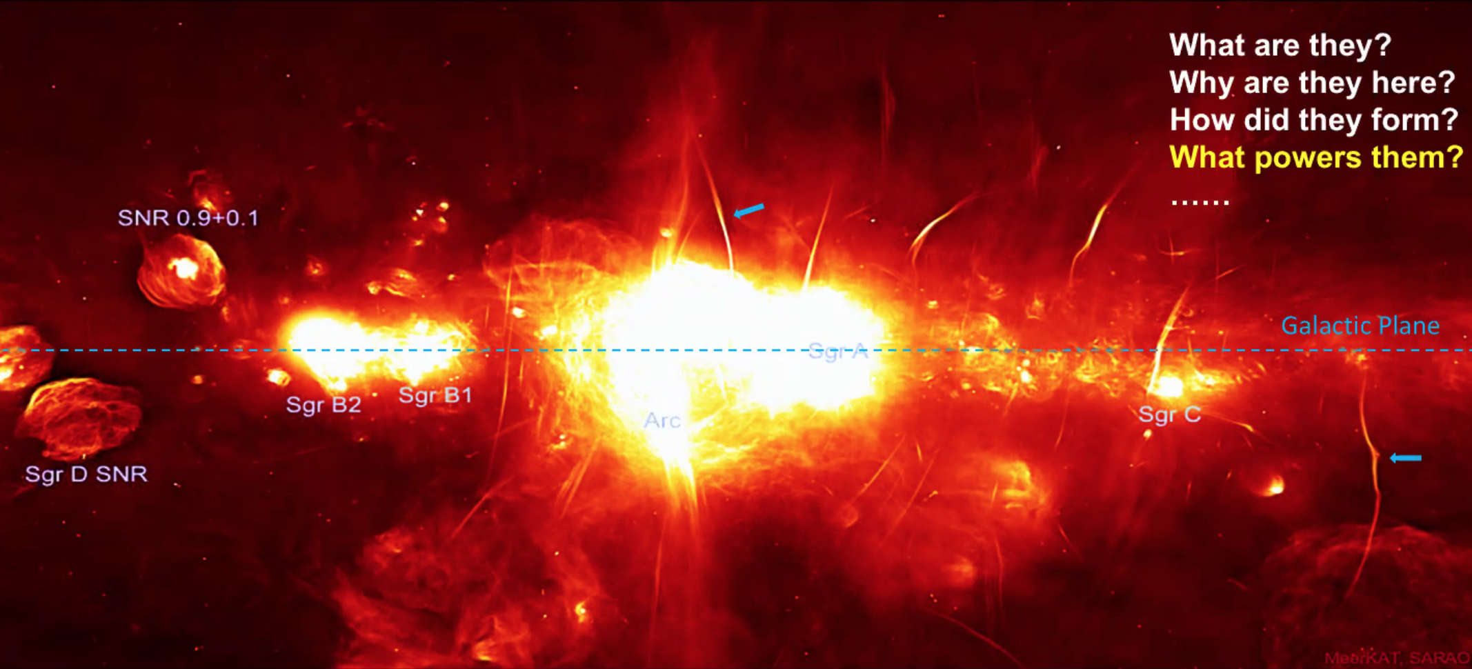
A look at our galaxy’s center in radio wavelengths reveals some curious features: long, thin filaments that span distances of up to hundreds of light-years, but are only a fraction of a light-year in width. What are these odd structures, and why do we see them? Shuo Zhang (Bard College) presents X-ray observations of several newly detected filaments that help us to answer this latter question. The new detections lead Zhang and collaborators to hypothesize that the filaments are lighting up in radio and X-rays as they’re bombarded by energetic particles accelerated in the galaxy’s core — possibly by the black hole Sgr A* itself. Press release
The galactic center contains mysterious filaments seen at radio and X-ray wavelengths. [Slide from Zhang; Image from MeerKAT/SARAO]
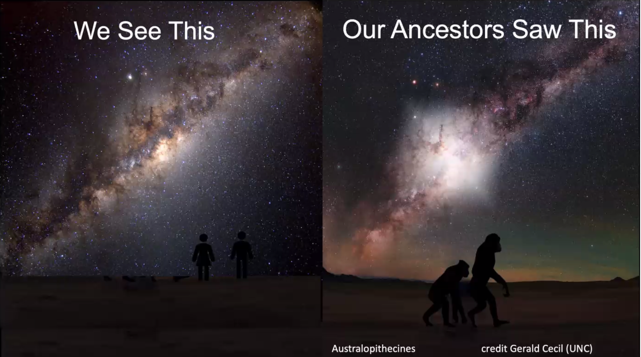
Closing out the session, Andrew Fox (Space Telescope Science Institute) presents an exciting possibility: though Sgr A* is quiet now, our supermassive black hole may not always have been so peaceful. Fox proposes that, just 1 to 4 million years ago, the galaxy’s center produced an enormous flash known as a Seyfert flare. This flash of light would have made the night sky look dramatically different for our ancestors millions of years ago! Fox shows that this theory is supported not only by the creation timeline for the Fermi Bubbles (a topic we’ll be touching on in greater detail in tomorrow morning’s press briefing), but also by evidence of photoionization in the matter that makes up the Magellanic Stream, a stream of gas that trails the Large Magellanic Cloud and may have been in the line of fire when cones of ionizing ultraviolet radiation erupted from the galactic center during the flash. Press release
An intense flash from the galactic center a 1–4 million years ago may have provided our ancestors with a very different night sky. [Gerald Cecil (UNC)]
Plenary Lecture: Satellite Mega-Constellations and the Night Sky: OIR Visibility, Impacts, and Policy; and An Introduction to the RF Spectrum Regulations (by Luna Zagorac)
The first half of this midday plenary was given by Dr. Sandra Cruz-Pol, a Program Leader at the National Science Foundation. Dr. Cruz-Pol underscored the importance of radio frequency (RF) signal management by explaining that if our eyes were able to see all the radio signals that surround us, we couldn’t see farther than a few meters. Furthermore, without regulation of RF channels, all of our communication devices would be rendered unusable due to interference — including cell phones, satellite TV, GPS, hurricane tracking, and more! After all, the RF spectrum is a limited resource, and radio regulations are constantly changing to keep up with new technologies.
Radio regulations exist at both the international and national levels. Since satellites regularly cross borders, their feeds need to be regulated internationally through the International Telecommunication Union, a UN agency. The ITU splits the world into three regions (with the Americas constituting Region 2), and holds the World Radiocommunications Conference (WRC) every 3–4 years in Geneva. The conference lasts for 4 weeks, and produces both radio regulations via international treaty, which all signatories must abide by, and recommendations, which are typically not mandatory. Nationally, federal assignments are handled by the National Telecommunications Information Administration (NTIA), and non-federal cases are handled by the Federal Communications Commission (FCC). In order for the FCC to adopt a proposal to change RF spectrum regulations in the US, a three-step process is necessary.
The NTIA also publishes the Frequency Allocation Table (FAT), which shows the signals at each frequency band, including primary allocations in capital letters and secondary allocations in lowercase. Primary allocations grant specific services priority in using the allocated frequency band; if there is more than one, they have equal rights, and have a right to be protected. Secondary allocations involve services that are allocated the same band as primary allocations, but must act to protect and accept interference from primary allocations.
In order to keep up with federal and international regulations, many organizations have Spectrum Managers — including Boeing, Nokia, Google, NASA, NOAA, the Navy, and more. NSF has two Spectrum Managers, who can be contacted for assistance with frequency assignments or questions at ESM@nsf.gov. Spectrum Managers also have to keep up with the many acronyms of various RF services — such as RAS (radio-astronomy service), SRS (space research satellite service, including near-Earth), ISS (inter-satellite service), and more.
Dr. Cruz-Pol closed by noting that RF allocation is a complicated topic on which she teaches an entire course, and so many details were left out of her presentations. She also provided listeners with an overview of free resources available online for those interested:
After that, Mary Elizabeth Moses Professor of Astronomy James Lowenthal of Smith College began his address with solidarity with those suffering from distress over recent events, especially the death of George Floyd and the longstanding harm of institutional racism and police brutality in the US. He then proceeded to show an image of a trail of StarLink satellites, stating: “My life as an astronomer changed early last year when I saw this for the first time.” The launch of StarLink satellites began in 2019, and a total of approximately 1,600 StarLink satellites are scheduled to be in the sky by the end of 2020. The satellites are launched into Low-Earth Orbit (LEO), starting at about 300 km and reaching their final altitude of about 550 km. They are relatively big satellites, about 3.5 by 8 meters long, and they are meant to provide fast broadband low-latency internet coverage worldwide.
The total number of objects in LEO is close to 20,000, consisting mostly of fragmentation debris, which is generated when larger objects collide and fragment into small pieces — intentionally or otherwise. However, most of these objects are not visible to telescopes and are far from visible to the naked eye. This is not true of StarLink satellites, which have elements that reflect sunlight to Earth and have a brightness magnitude less than 5, most noticeably around morning and evening twilight. The satellites have three phases of life — launch and orbit raise (1–6 weeks), operation (5–25 years), and de-orbit — all of which can impact observations, and different satellites might be in different phases concurrently. Modelling from the Vera Rubin Observatory (formerly LSST) showed that on the night of the summer solstice in Chile, 1–9 StarLink satellites would be visible to the observatory at twilight if orbitingat ~500 km. If the satellites were raised to 1,150 km altitude (still technically LEO), 10–25 satellites would be visible all night long.
The brightness of the satellites can completely saturate the CCDs of the VRO, leading to tracks of corrupted data. Furthermore, if they are bright enough, they can produce “ghost trails” that are impossible to correct for in the data, rendering more of the image unusable. With the current number of StarLink satellites, VRO can dodge some of these trails in its field of view, but as the numbers rise this will become impossible. Furthermore, some telescopes with wider fields of view are already unable to do this.
This is a major collision of technologies: the new advanced land-based telescopes and satellite mega-constellations. Dr. Lowenthal notes that, as described by Dr. Cruz-Pol, the protection of the radio sky has been a fortunate fact for decades; however there is no such protection for the optical/infrared sky. While the launch of a satellite requires permissions from many agencies, including the FCC, FAA, and ITU, it decidedly does not require permission from the AAS, the International Astronomical Union, or the International Dark-Sky Association. To suss out the impact of these mega-constellations, the AAS sent out a survey in December 2019 and got answers from all seven continents, including astronomers at observatories like VRO, Gemini, VLT, ZTF, APO, ATLAS, Las Campanas, and more. The answers for current impacts reported a wide range of 0–100% of science lost, with the majority expressing significant concerns, and in some cases significant costs. In the projection of 20,000 more bright satellites (compared to 1,584), 17/23 respondents noted that virtually all their science would be impacted, with 12/23 projecting critical failure of the facility.
The AAS has been in conversation with satellite operators (primarily SpaceX), and CEO Elon Musk has committed to reducing StarLink’s impact on science to zero. There have been several attempts to minimize brightness, including painting the satellites black (DarkSat), equipping them with visors to shield from sunlight (VisorSat), and re-orienting them so that the sunlight falls on the knife-edge of the satellite, minimizing reflection. However, other operators are planning to launch LEO satellites in the near future, prompted by a $20 billion subsidy from the FCC for such activities, and there is no guarantee that they will be as collaborative as SpaceX.
Finally, Dr. Lowenthall voiced his opinion, which is that astronomy is facing its most serious threat ever in LEO satellite mega-constellations. He further reflected on the impact of the sky to the human experience, including what the stars and the sky are worth; whose sky is it and who decides; what the value of exploring the cosmos is; and if there are viable alternatives to LEO satellite mega-constellations. Last, he emphasized that the impact of these constellations on the ecosystem is not known, but should be explored — for example, with respect to migratory birds using the stars to navigate. He encouraged astronomers to promote and lead such discussions internationally and with multiple stakeholders, and he then finished with a time-lapse from his own backyard in Massachusetts, asking attendees to spot the StarLink trails.
Dr. Lowenthal ends with this image taken from his home and asks us to to spot the starlink satellites… #AAS236pic.twitter.com/oOygnn2imG
National Science Foundation (NSF) Town Hall (by Tarini Konchady)
The National Science Foundation (NSF) town hall featured Ralph Gaume, Director of the Division of Astronomical Sciences (AST); Jim Neff, AST Deputy Division Director; and B. Ashley Zauderer, an AST Program Director whose programs include the Arecibo Observatory and Electromagnetic Spectrum Management.
Gaume’s presentation focused primarily on the impact of COVID-19 on AST and the NSF. A number of NSF-managed observatories have been operating through the pandemic, specifically the National Radio Astronomy Observatory facilities, Green Bank Observatory, Arecibo Observatory, the Global Oscillation Network Group, and Gemini North. The facilities currently idle are Gemini South, the Cerro Tololo Inter-American Observatory (CTIO), ALMA, and the Kitt Peak National Observatory (KPNO). Construction on the Vera Rubin Observatory (VRO) and the Daniel K. Inouye Solar Telescope (DKIST) has also paused. Many of the stalled facilities will require significant work to bring back online, with ALMA in particular posing an enormous challenge. The roadmaps for the next few years regarding VRO and DKIST will also have to be reworked.
The results of the Decadal Survey will also be presented later than anticipated, but the NSF transitioned very smoothly into teleworking right from March. Gaume also mentioned personnel changes in AST and the NSF as a whole. Most notable is the end of France Córdova’s term as NSF Director on March 31 this year. Her likely successor is Sethuram Panchanathan, who was nominated by the President in January. While Panchanathan’s nomination makes its way through Congress, Kelvin Droegemeier (who will be at an AAS 236 town hall tomorrow) has been serving as Acting NSF Director. Droegemeier is also Director of the Office of Science and Technology Policy, which advises the White House.
Gaume wrapped up by highlighting science from the NSF’s facilities, including the new NSF’s National Optical-Infrared Astronomy Research Laboratory — NOIRLab for short. NOIRLab was founded on October 1 last year and consists of all the NSF’s nighttime ground-based observatories in addition to the Community Science and Data Center. The rest of the science highlights can be found in the Twitter thread linked below:
The NSF's new telescope has taken the highest resolution ground or space-based image of the Sun ever taken by humans; resolution is a few tens of kilometers! pic.twitter.com/z7lChwnXEA
On the budget side, AST and the NSF are doing reasonably well. As usual, the President’s Budget Request for the fiscal year 2021 decreased NSF funding, but also as usual, Congress appropriated funds for the NSF at a level higher than the Request level. Legislature to watch includes the Securing American Leadership in Science and Technology Act, introduced by Republicans on the House Committee of Space, Science, and Technology, and the Endless Frontier Act, spearheaded by Senate Minority Leader Chuck Schumer. The latter would significantly change the operations of the NSF and other federal organizations.
Gaume then handed things off to Neff, who focused on the status of various AST grants. Neff emphasized that the grants and programs under AST were heavily informed by community input. The pandemic has caused disruptions to several grant programs, but AST is working to remedy this. Astronomy and Astrophysics Research Grants are currently being awarded with a success rate of roughly 1 in 5, which is standard. Neff reminded attendees of the deadlines for different AST grants as well as grants in other divisions that astronomers could be eligible for. These grants include opportunities in data science and computer engineering. Neff wrapped up by introducing the new guide to NSF proposals and research.gov as a resource.
Zauderer wrapped up the town hall by discussing the NSF’s efforts on protecting spectrum use for astronomy. She referred attendees to the plenary by Sandra Cruz-Pol and James Lowenthal earlier today for a deep dive into the issue. The NSF would like to expand its efforts in radio spectrum management and extend these efforts to optical wavelengths. Zauderer mentioned that private companies like SpaceX have been amenable to mitigating harm to astronomy. To that end, she highlighted the Satellite Constellations 1 Workshop, a joint effort between the AAS and NOIRLab that will bring together “astronomers, satellite operators, dark-sky advocates, policy-makers,” and others to discuss the impact of satellite constellations. She also highlighted the NSF’s Spectrum Innovation Initiative, which would offer funding to parties interested in this issue.
Space Telescope Science Institute (STScI) Town Hall (by Amber Hornsby)
Opening the Space Telescope Institute (STScI) town hall today was the director of STScI, Dr. Kenneth Sembach, who started with a general update of operations. The key take-away message from the director is, “we are here to support and help you advance scientific discovery.” Naturally some activities have been impacted by COVID-19, but things are slowly starting up again with seminars, proposal evaluations, and more being re-imagined for online platforms.
Next on the agenda for Sembach was discussion of a very exciting project — the Ultraviolet Legacy Library of Young Stars as Essential Standards (ULLYSES). With a grand total of 1,000 orbits, this is the largest single Hubble Space Telescope (HST) program ever executed, and it has two primary objectives: (i) 500 orbits to extend the spectroscopic library of O and B stars of low metallicity and (ii) 500 orbits to create a spectroscopic library and time monitoring of T-Tauri stars (younger than 10 Myrs). The first data release of the Small and Large Magellanic Clouds will be in September 2020.
Illustration of NASA’s WFIRST telescope, now the Nancy Grace Roman Space Telescope. [NASA]
The final, and possibly most exciting, part of Sembach’s talk was presenting the Wide Field Infrared Survey Telescope (WFIRST) as the Nancy Grace Roman Space Telescope. “NASA could not have chosen a better person,” said Sembach, because “she loved the universe.” This is where the STScI and NASA asks for help from the community. “We want and need to know how you will use the Nancy Grace Roman Space Telescope.” Please participate in an open community survey by June 15.
Moving on to a big problem in modern astronomy — Dr. Joshua Peek discussed large data sets and improving their accessibility. As new instruments come online and take an unprecedented amount of data, it becomes more and more challenging to ensure everyone can access the archived data and that they can do exciting science with it. STScI has already started tackling this problem with a NASA-funded project, the Milkulski Archive for Space Telescopes (MAST), which collates data from the HST, the Transiting Exoplanet Survey Satellite (TESS), and Kepler.
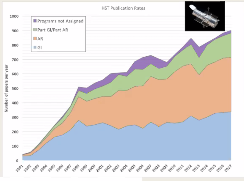
Data are getting BIG, now over a petabyte. Number of institutions per paper is also growing, the median is now five! #AAS236pic.twitter.com/jK0K7XtaFj
So far, astronomers are already making great use of MAST to write an impressive number of papers, which has highlighted another trend in astronomy: the number of institutions represented on a paper. The median number of institutions for every paper published using MAST data is now 5. This represents another problem facing many groups: the problem of each member being able to access data sets and work on them simultaneously. Here, Peek introduces the Time series Integrated Knowledge Engine, otherwise known as T.I.K.E.
T.I.K.E is a public, cloud-based Jupyter lab environment which contains pre-installed software for interpreting time series data, the kind associated with the study of exoplanets. Not only are your usual python packages like Numpy and Scipy built in alongside key packages for astronomy, like Astropy, but T.I.K.E also includes specialised packages created to work with time series data such as Exoplanet. All of this is useful, but what makes T.I.K.E next-level is access to TESS and Kepler data through the platform, the built-in notebooks and shared repositories for collaborations. Through T.I.K.E, the learning curve to participate in astronomy will be reduced, which will “accelerate science” and enable scientists to “find more stuff”, more quickly. T.I.K.E will be available sometime this summer.
Next up, Dr. Karoline Gilbert presents ‘Hundreds of Hubbles in the 2020s: realising the scientific potential of the Roman Space Telescope Archive’. Having recently passed the “formulation” phase of the mission, we’re now moving towards “implementation,” meaning the design has been finalised, thus hardware is now in development, and flight detectors are being built and delivered.
With a Hubble-sized primary mirror of 2.4 meters, we can already anticipate beautiful Hubble-quality images from the Roman Space Telescope when it is launched within the decade, but what is particularly revolutionary is its field of view. Having a larger telescopic view allows large areas of sky to be mapped faster. For example, the Roman telescope can measure the complete satellite and cluster populations of a galaxy, capturing the extent of the dark matter halo, with Hubble-like sensitivity and resolution in one pointing. For nearby galaxy surveys, like the Panchromatic Hubble Andromeda Treasury (PHAT), the Roman Telescope can map the same region almost 1,500 times faster.
Furthermore, data from the Roman Space Telescope will be publicly available with no proprietary period, via a T.I.K.E-like environment. This is an exciting step forward towards a more open and accessible field of astronomy, which will enable an impressive amount of science to be done by astronomers all over the globe. Currently, the team predicts proposal opportunities will be available at the beginning of 2021 and invites astronomers to participate in a virtual conference focused on the future of galaxy formation and evolution studies in October.
To close out the town hall, Dr. Louis Strolger reports on the recent HST proposal cycle 28 and the changes implemented in the review process. To address the COVID-19 impact, the proposal deadline was extended and the review was completed entirely via virtual platforms. Another recent change that also occurred for the last two cycles was a dual-anonymous review hiding the identities of proposers throughout the scientific ranking phase. This process is having an important impact on the gender diversity of proposers.
Over the last three cycles, the gap in proposal acceptance rate between male and female PIs has decreased from an average of 5% to 1%, with a predicted increase of female-led proposals of 0.5% per year. Furthermore, the number of PIs being awarded programs for the first time is also on the up, suggesting the dual-anonymous process is allowing the next-generation of scientists to get telescope time. Due to its success, the dual-anonymous review process will continue to be implemented and will also be used for James Webb Space Telescope (JWST) proposals, which are expected to be due in late fall.
Press Conference: Planets, Exoplanets & Brown Dwarfs (by Haley Wahl)
The second press conference of the day focused on planet-like objects!
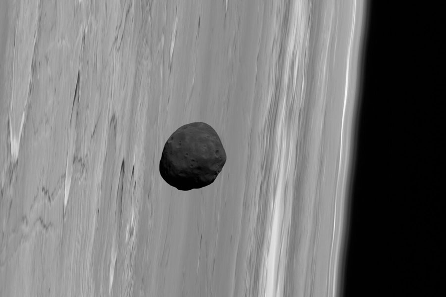
Phobos as seen by Mars Express. [G. Neukum (FU Berlin) et al., Mars Express, DLR, ESA; Peter Masek]
First up was Matija Cuk from the SETI Institute speaking about Mars’s moons. The planet Mars has two moons: Phobos and Deimos, both of which were previously thought to be captured asteroids. However, by looking at the orbital inclination of Deimos, this team found evidence of a past Martian ring that created what is now Phobos — and that ring was formed from a “proto-Phobos” which was 20x the current mass of Phobos. This, his team believes, is only the latest case in a cycle of a moon becoming a ring and then the ring becoming a smaller moon. Press release
Next up was Fritz Benedict from the University of Texas, Austin to talk about calculating the mass of the recently identified, nearby planet Proxima Centauri c. By revisiting 25-year-old Hubble data, combined with some newer results from 2020, his team finds that the mass of Proxima Centauri c is either that of 18 Earths or 7 Earths, depending on which measurements are included in the calculations. Though there is still work to do, this finding shows that you can indeed find new results from old data. Press release
The third speaker was amateur astronomer Paul Benni from the Acton Sky Portal. He discussed the first discoveries of the Galactic Plane Exoplanet Survey (GPX). The first of these new discoveries is KPS-1b: the first transiting exoplanet (a hot Jupiter) discovered using an amateur astronomer’s wide-field CCD data. Another major discovery was GPX-1b, a transiting brown dwarf orbiting an F star. This was not detected by TESS algorithms because the host star was <1 arcmin away from a really bright star, so it diluted away the transit signal. The final discovery: a pre-cataclysmic binary with unusual chromaticity of the eclipsed white dwarf! Read more about Paul’s work in his paper.
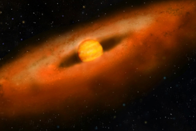
Illustration of a brown dwarf surrounded by a disk. [NASA/William Pendrill]
The final speaker of the press conference was Maria Schutte (@maria_schutte), a PhD student at the University of Oklahoma. She discussed the citizen science project Disk Detective, which allows people at home to find new planet-like systems. This project led to the discovery of W1200-7845, an especially young (~3.7 Myr), nearby (332 light-years) brown dwarf disk! W1200-7845 provides us with a unique opportunity to study a potentially planet-forming disk around a nearby brown dwarf. To learn more, follow @diskdetective on Twitter. Press release
Plenary Lecture: The Atacama Cosmology Telescope and the Simons Observatory: The Millimeter-Wave Sky from Chile (by Amber Hornsby)
For the final plenary of day 2 at AAS 236, Prof. Jo Dunkley (Princeton University) presents the millimeter sky as viewed by the Atacama Cosmology Telescope (ACT) in Chile, and plans for a next-generation cosmology telescope, the Simons Observatory (SO). Throughout the plenary, there is a focus on the cosmic microwave background (CMB) and what it tells us about the universe; however, we also learn about bonus discoveries that can be made with detailed surveys of the millimeter sky.
The CMB is often referred to as the “afterglow of creation” because we’re looking at the oldest photons in the universe. Initially, the universe was a hot, opaque soup of interacting photons and baryons. After 380,000 years, the universe had expanded and cooled enough for photons to escape, and this is the remnant light we can observe today. When observed for the first time in 1964, it appeared to act like a perfect, uniform blackbody with a peak temperature of 2.74 K and peak wavelength of around 2 mm. But, thanks to improved measurements, we now know there are actually tiny temperature fluctuations in the CMB.
The best known, most recent image of the CMB is from the Planck Satellite. We see the seeds of our large scale structure from fluctuations in the primordial plasma. Isn't out baby universe cute? #AAS236pic.twitter.com/omKzsfSvZk
The temperature map, created using data from the Planck space telescope, is a nice snapshot of the physics of the universe at a redshift of z = 1,100. The intensity of the CMB mainly tells us about the density of the photon-baryon plasma, where hot spots (shown in red) represent denser regions. Dunkley explains how, if the map is decomposed in terms of angular scale, we can plot the amount of “bumpiness”, the so-called power spectrum of the sky. Given this, we can theoretically predict different model universes, containing different initial ingredients and conditions until our predictions fit the observed data. The best-fit model to Planck data is given by a Lambda-Cold-Dark-Matter (LCDM) cosmological model requiring three ingredients and two initial conditions.
The CMB is a backlight to every other signal we see, and so it sensitive to universe effects, including lensing, the tSZ, and the kSZ. #AAS236pic.twitter.com/PxIfzN7fdw
As CMB photons travel through the universe, they encounter galaxies, hot electrons and more, which alter the photons in some way. For example, CMB photons are very sensitive to massive objects, which results in the lensing of the CMB. It is further distorted by the thermal and kinetic Sunyaev-Zel’dovich (SZ) effect. The thermal SZ effect is where hot electrons scatter the CMB, causing a shift in its observed spectrum, whilst the impact caused by the momentum of high-energy electrons is characterised by the kinetic SZ effect. It is important to characterise these effects to get an accurate picture of the CMB.
However, something that CMB enthusiasts can forget is the “wealth of information” contained within surveys of the millimeter sky beyond the CMB. Dunkley points to observations of polarised dust taken by Planck. Although dust contaminates our CMB signal, we can infer the orientation of the magnetic fields in our galaxy through the alignment of dust grains by simply rotating the polarisation signal by 90 degrees. This is because dust grains align themselves perpendicular to the magnetic field. But this is only the start. Surveying the millimeter sky addresses other key astrophysics questions, such as (i) how long did reionization take? (ii) where is Planet 9? (iii) is the accelerated expansion of the universe just Lambda?
Dunkley now introduces ACT, and how it builds on Planck’s legacy. ACT has been operating since 2007 and its third-generation instrument has around 5,000 detectors. There are a few differences between ACT and Planck, such as ACT only mapping 40% of the sky and being ground-based. However, ACT data have 3 times less noise than Planck data and are much better resolved. In recent ACT maps, this has uncovered radio galaxies (blazars) and galaxy clusters through the SZ effect. Moreover, ACT has observed the largest-ever SZ galaxy cluster sample containing over 4,000 clusters!
ACT also adds to resolution in the polarization signal — here, the E-field polarization is shown. White is less and black is more polarized than average. Though it looks noisy, we really can see fluctuations in velocity from the early universe. #AAS236pic.twitter.com/ky6qy5LJgH
Additionally, ACT has captured unprecedented views of the polarised sky at 2 mm, the signal size of which is known as the E-mode component of polarisation. Here, white represents higher polarisation on the grey-scale image. We can also create a power spectrum based on ACT data which, combined with data from the ground-based telescopes POLARBEAR and the South Pole Telescope (SPT), can provide an independent calculation of the contentious Hubble constant. A paper on this new result is currently in preparation.
Sadly, Dunkley reveals, we have hit an upper limit on the number of detectors we can fit in the telescope. This is important because without more detectors, we cannot make further reductions in the noise in our observations. We thus need to consider a new telescope — Simons Observatory. Already under construction, the 6-meter-primary telescope will live alongside ACT in Chile and will house over 30,000 transition-edge sensor detectors.
This impressive telescope will have a huge impact on the millimeter community, providing new opportunities to participate in transient science through synergy with multiple surveys. SO plans to track thousands of variable active galactic nuclei on a daily/weekly/monthly basis at 1–10 mm wavelengths. With an observing timeline of 2023–28, SO will overlap with the Vera Rubin Observatory, the Dark Energy Spectroscopic Instrument (DESI), and Euclid, enabling observations to be completed simultaneously at different wavelengths. In addition to the substantial improvements in CMB observations, including the potential for a glimpse of the elusive B-mode component of the polarised CMB, SO will also observe 30,000 high-redshift, dusty galaxies and 20,000 clusters.
In her closing remarks, Dunkley reminds us that there is “so much to learn from wide-field surveys of the millimeter sky.” We can learn about our galaxy, transient sources, AGNs, and my favourite, the CMB, which gives us a “unique view of the early universe.” ACT scientists are looking forward to sharing new data and software with the astronomical community — so keep an eye out for upcoming press releases.
Editor’s Note: This week we’re at the 236th AAS Meeting, being conducted virtually for the first time! Along with a team of authors from Astrobites, we will be writing updates on selected events at the meeting and posting each day. Follow along here or at astrobites.com. The usual posting schedule for AAS Nova will resume the week of June 8th.
Welcome Address (by Sanjana Curtis)
AAS President Megan Donahue (Michigan State University) kicked off the 236th meeting of the American Astronomical Society — the first AAS meeting that is entirely virtual. Before opening the meeting, she acknowledged the fact that many members of the astronomy community are not present due to a variety of factors, including a pandemic, the choices of others, and an uninterrogated system that grants privileges to a select few. This was a sobering reminder that science is, above all, a human endeavor.
As a virtual meeting, this AAS has a low carbon footprint that is certainly good news for the environment. At the same time, the meeting attendance is almost double the usual attendance at in-person meetings, including twice as many students! There are scientists from 34 countries and 49 of the 50 US states (with the exception of Alaska) in attendance. The schedule is packed, the science is exciting, and we’re looking forward to 3 days of hearing about the latest research and the newest results in astronomy!
AAS President Megan Donahue’s welcome acknowledgements.
Fred Kavli Plenary Lecture: Searching for Habitable Worlds: Challenges, Opportunities & Adventures (by Sanjana Curtis)
Lisa Kaltenegger (Carl Sagan Institute) delivered the Fred Kavli Plenary Lecture and spoke about the challenges, opportunities, and adventures to be found in our search for habitable worlds. Starting from being able to observe just a handful of exoplanets, we have now reached a point where we can start doing statistics with them. We have found thousands of new worlds that show great diversity in their properties, and exploring this diversity through theoretical modeling can help us understand the physics of both the planets and their host stars. A wonderful review on this topic can be found here.
Kaltenegger presents a radius vs. mass plot of measured exoplanets. Click to enlarge.
Dr. Kaltenegger also addressed whether we can distinguish the population of rocky planets from the population of gas planets based on the mass and radius of the exoplanet. If we know both the mass and the radius of an exoplanet, we can derive its mean density and composition, and compare it to planets in our solar system. However, for most exoplanets, either the mass or the radius is known depending on the detection method. In general, the line dividing gas planets from rocky planets sits at around 2 Earth radii—all exoplanets below this limit are rocky planets.
Kaltenegger’s group has created a catalog of exoplanet spectral fingerprints.
The spectra of exoplanets are key to understanding their properties and Dr. Kaltenegger’s research group is creating a database of spectral fingerprints to compare against future observations by telescopes like ELT or JWST. These data are freely available here. She stressed that we do not just have the current Earth as a template for habitable planets, but also the Earth through time.
She ended her talk with some intriguing and adventurous ideas: the possibility that organisms on planets around active M stars may develop biofluorescence to protect themselves from harsh ultraviolet light, and the existence of habitable worlds around red giants and white dwarfs!
The second press conference of the day involved new studies on some galactic oddities! Four scientists took turns sharing what they’ve discovered lurking in our cosmic neighborhood.
Satellite galaxies of NGC2998 have a “lopsided” distribution. This image shows how there seem to be more satellite galaxies (circled in yellow) on one side of the host galaxy (circled in blue) than the other.
First, Tereasa Brainerd (Boston University) shared her team’s findings that involved the distribution of satellite galaxies around a host galaxy. Scientists believe that the dark matter halos that surround galaxies (as predicted by the cold dark matter theory) are spherical, flattened elliptical halos. By looking at the systems with 5+ satellites around the host galaxy, they found “lopsided” distributions, meaning there were more pairs of galaxies on one side of the galaxy than the other. Could this have implications for cold dark matter? It’s possible!
Next up was Lior Shamir (Kansas State University) who continued the theme of asymmetries. He presented observations that showed that the distribution of apparent spin directions of galaxies isn’t always symmetric, that it changes depending on the direction of observation. He also showed that the direction of spin is linked to its brightness and that asymmetry varies with redshift. Press release
The extent of the hot circumgalactic medium around the galaxy studied by Das’s team.
The third speaker was Sanskriti Das (Ohio State University), who talked about evidence for a massive hot circumgalactic medium around a luminous star-forming galaxy. She and her team showed, using X-ray data, that this material, which is extended over a large volume and has a large mass (comparable to the mass of all the stars in that galaxy!), could be the solution to the “missing baryons” problem in galactic halos. Press release
The last speaker of the press conference was Ripon Saha (University of Missouri, Kansas City), who presented the discovery of a massive proto-supercluster 10 billion light-years away. Using a pipeline made using dust-obscured galaxies (DOGs), he and his team identified the proto-supercluster of galaxies surrounded by nascent ones. This is the first time any observed cluster has been found embedded in its birth environment, which could give astronomers a unique opportunity to study such a cluster.
Plenary Lecture: The Inclusion Revolution (by Luna Zagorac)
The midday plenary entitled “The Inclusion Revolution” was delivered by Dr. Dara Norman, the Deputy Director of the Community Science and Data Center at NSF’s NOIRLab in Tucson, AZ. Dr. Norman began her plenary by describing the term “culture”: the customs, institutions, and achievements of a group of people. As scientists and astronomers, we have our own culture — including our language, our traditions, our norms, our values, and even our art — and parts of this culture must be changed to support diversity and inclusion in astronomy. Indeed, culture is not a static object: an example of cultural change comes from the very first decadal survey, which addressed the demographics of the workforce and the lack of availability of public telescopes. This led to the funding of the national observatories, without which the state of astronomy today would look completely different, underscoring the potential impact of the 2020 and future decadal surveys.
The AAS decadal survey has always been a tool for assessing the demographics of astronomers conducting research, and for changing culture. Indeed, the first one ever published fueled the founding of national observatories due to lack of access to telescopes nationwide!
A point that Dr. Norman emphasized throughout her plenary is a quote from Paula Stone Williams’s TED talk — “I didn’t know what I didn’t know.” The first step towards inclusion is thinking about not just who is represented on policy-making committees, but what kind of expertise is represented. It’s not enough to have a lot of different voices if there isn’t a critical mass of expertise in the room. Additionally, we need to empower each representative to act as a mouthpiece for their community, while gathering ideas and thoughts from the community. In this way, the issue of having too many people on committees can be avoided, and the workload redistributed amongst individuals.
The blue area represents the papers written on data from dedicated HST observing runs, while the orange represents papers from archival data. Note that the numbers equal out with time!
Next, Dr. Norman discussed her paper (Norman 2018), which explored how to use big data to reach insider status in the field — including being invited to join collaborations, give talks, review papers, and more. She found that, with time, the number of papers published on data from allocated Hubble time evened out with the number of papers written from archival data. Findings from Peek et al. (2019) broke that down by authorship, and the gap was significantly larger at small and underfunded institutions. This raised the question of whether archival data can be used as a vehicle to accessing the dedicated observation time that is critical for advancing in the field.
Figure from Peek et al. 2019. The blue line represents HST papers published using archival data, while the orange represents papers stemming from dedicated observing time. Note the discrepancy between large and small institutions!
Dr. Norman is looking for a 3-year postdoc (click to enlarge)! The posting is not out yet, but you can contact Dr. Norman via email for more details.
Going back to the general theme of “you don’t know what you don’t know,” the first step to bridging this gap is to directly ask colleagues at small and underserved institutions what they need. One of the needs Dr. Norman identified was the need for more policies and incentives for R1 institutions to work with smaller institutions, as is currently rarely the case. To this effect, Dr. Norman will be working on a toolkit for effective diversity and inclusion practices and their efficacy, particularly aimed at underserved institutions. She will be looking for a 3-year postdoc to aid in this effort, and can provide more information upon email request.
Dr. Norman ended her talk by underscoring that there is much more work to do on diversity and inclusion in astronomy, including through the decadal surveys, which have been a tool for demographics-driven cultural change from the very start. She closed by reminding us that we need change; that the revolution will not simply be tweeted; that black lives matter; and to vote.
NASA Town Hall (by Abby Waggoner)
The NASA Town Hall was led by Paul Hertz, Director of the Astrophysics Division in the Science Mission Directorate at NASA. The NASA Town Hall provided an overview of NASA operations, funding, and missions from the past year, along with goals and funding for the future. Below, each topic covered is summarized in bullets. All images are obtained from the slides provided during the town hall.
Where does NASA Astrophysics funding go? The numbers shown in this figure shows that the funding goes to supporting many scientists and projects!
Committed to Improving
Mission PI Development: NASA seeks to increase the diversity of mission principal investigators.
Fellowships and funding for graduate students and postdoctorates were awarded, including:
Nancy Grace Roman Technology Fellowship
Hubble Fellowship
NASA Earth and Space Science Fellowship (NESSF)
Future Investigators in NASA Earth and Space Science Technology (FINESST).
Peer reviews have become anonymous.
Mission Program Update
Impact of COVID-19: Flight operations have continued nominally with the exception of the Stratospheric Observatory for Infrared Astronomy (SOFIA has been grounded; see below).
Priority has been given to Mars 2020 and the James Webb Space Telescope (JWST).
Updates from missions currently in flight:
Hubble had its 30th birthday. You can find out what Hubble was imaging on your birthday here.
The Transiting Exoplanet Survey Satellite (TESS) has discovered 47 confirmed planets and 1,837 planet candidates. The four-planet system HD 108236 was highlighted, as the three outer planets are candidates for spectral analysis with JWST.
SOFIA has suspended flight operations since March 2020 due to COVID-19. There will be a community update on SOFIA on June 2 at 3pm (EDT) during AAS 236.
NASA has 10 missions planned for the future. These missions include a science goals ranging across the entire electromagnetic spectrum.
Updates from among NASA’s 10 missions currently in development:
JWST has undergone deployment testing, and will soon begin observatory-level environmental testing.
Roman Space Telescope (formerly Wide-Field IR Survey Telescope, or WFIRST) is fully funded and in production. Roman will aid in understanding the evolution of the universe to exoplanet direct imaging.
Two small explorers are planned:
ESCAPE will investigate UV stellar flares and their impact on the habitable zone.
COSI will observe MeV gamma-rays to trace the Milky Way’s supernova activity.
Two missions of opportunity are planned:
Dorado will watch for UV light emitted by merging neutron stars.
LEAP will be attached to the ISS and observe the polarization of gamma-ray bursts in jets.
NASA funding for the 2020 year and how the funding is being allocated.
Planning for the Future
NASA funding for the Astrophysics Division is at an all time high, with 58% of the funding dedicated to JWST and Roman.
NASA seeks to have humans sent to the moon by 2024 through the Artemis Project.
In the next decade, NASA has concepts for several medium and large missions in the 2020 Decadal Survey.
Press Conference: Cosmic Bangs & Whimpers (by Alex Pizzuto)
Deborah Schmidt (Swarthmore College) kicked off this afternoon’s press conference by summarizing her dissertation work, which focuses on the abundance of different atomic isotopes in planetary nebulae. While many of us may know of planetary nebulae, such as the butterfly nebula, for their strikingly beautiful silhouettes, these objects “also play a significant role in the recycling of matter in our universe,” according to Schmidt.
Planetary nebulae are the final stages of Sun-like stars. Towards the end of their lives, stars can eject material that flows away from the remnant core and enriches nearby interstellar regions, filling it with a wide array of elemental isotopes that were originally produced in nuclear reactions within the star. Until recently, it was thought that these isotopes shouldn’t linger very long, because the hot white dwarf remnant at the center of this nebula should produce a plethora of high-energy radiation, which has the potential to destroy the expelled molecules.
Schmidt presented recent radio observations that challenge these beliefs, and found that these regions, although expected to be cleared out of these elemental abundances, were instead “bursting with molecules.” This wealth of elemental isotopes was found in both the young and old nebulae that Schmidt studied, and this discovery has major implications for a breadth of topics. These include potentially remedying tensions relating to the prevalence of poly-atomic ions in the diffuse interstellar medium, as well as explaining the previously anomalous origins of dust grains that are present even in our own solar system. Additionally, these observations allowed Schmidt and collaborators to build a new model of the inner workings of planetary nebulae, and to show how potentially explosive origins can not only explain the prevalence of a variety of elemental isotopes, but can also explain the gorgeous shapes of planetary nebulae that we know and love.
Schmidt describes the plethora of elemental isotopes that originate in planetary nebulae and explains how these objects explain the anomalous abundances of elements in the diffuse interstellar medium.
Adelle Goodwin (Monash University) then went on to describe recent observations of extremely energetic outbursts visible across nearly the entire electromagnetic spectrum: accreting pulsars. Accreting pulsars consist of neutron stars, the dense remnants of dead stars, in close orbit with a “normal” star. Neutron stars are so dense that a mere handful of their material would have the same mass as about 5 Mount Everests, or 5 billion tons. If in orbit with a nearby star, these neutron stars can slowly consume their companions, filling up accretion disks until reaching a critical threshold, and then quickly gobbling up some of this material and expelling a fraction of it in a violent outburst.
Artist’s impression of an accreting pulsar. [NASA]
This outburst should be visible in a variety of electromagnetic wavelengths, including optical, UV, and X-ray, and the evolution of the radiation in these different wavebands reveals a wealth of information about the underlying processes that are occurring. Goodwin describes the first ever set of observations of this entire outburst period with simultaneous coverage in these various wavelengths. Specifically, her team targeted a pulsar located 11,000 light-years away, spinning 400 times per second, and they observed this pulsar with more than 7 telescopes. As Goodwin and her team investigated this object, they noticed that the X-ray emission began at a time much later than the optical emission, with a delay of about 12 days, longer than any model would have predicted. The team was able to reconcile this discrepancy by suggesting that the disk consists of a large fraction of helium, which takes longer to heat up and then ionize. Regardless of the delay of X-rays, these observations of an outburst thousands of times brighter than the Sun marks a new step in understanding the dynamics of these explosive transients. Press release
Next up was Justin Vandenbroucke (University of Wisconsin, Madison) on behalf of the Cherenkov Telescope Array (CTA), a team of scientists dedicated to investigating the universe at the highest energies. Some objects in our own galaxy are capable of producing particles of light with energies exceeding one tera-electronvolt (TeV), which is about one trillion times more energetic than the particles of light we detect with our own eyes. Studying this light, and the objects capable of producing it, teaches us about the most efficient and energetic accelerators in our universe.
In order to detect these particles, Vandenbroucke described a prototype ground-based gamma-ray telescope. When a gamma ray approaches the Earth, it can demolish an atom in the atmosphere. This collision produces a menagerie of particles travelling at nearly the speed of light, which in turn produce tiny flashes of blue light. The goal is to then reflect these tiny blips of blue light into a camera by building precise and gargantuan mirrors on the ground. In case that does not sound difficult enough, Vandenbroucke described how this telescope features a two-mirror design as well as state-of-the-art electronics. This symphony of advanced electronic and complicated optics should be able to come together to produce some of the most vivid and detailed pictures of the universe in its most energetic states.
To test out this new telescope, Vandenbroucke and his team pointed their telescope at the Crab nebula, the remnant of an exploded star from 1,000 years ago, which features a pulsar in the center powering very bright emission up to TeV energies. The team was able to significantly detect this object at these amazingly high energies. Vandenbroucke noted that this “detection establishes innovative telescope technology for gamma-ray astronomy.” Together with the other telescopes being constructed, the CTA consortium should revolutionize the way we see the universe and will play a pivotal role in both multi-wavelength and multi-messenger astronomy at the highest energies. Press release
Vandenbroucke shows the first detection of the Crab nebula with this revolutionary high-energy gamma-ray telescope, providing a picture of this object at energies trillions of times more energetic than we detect with our eyes.
Wrapping up today’s press conference was Fabio Pacucci (Black Hole Initiative & Center for Astrophysics), discussing how black holes grow. We know that black holes come in a variety of masses, ranging from those just a few times more massive than the Sun all the way to millions of times more massive than this. What we don’t know is how these black holes get to be so large.
Fabio Pacucci’s conclusions for how black holes of different sizes grow at different times in the universe. Click to enlarge and read text. [Illustrations: M. Weiss]
Fundamentally, there are two ways a black hole can acquire more mass: either they slowly accrete matter from their nearby environments over time, or they merge with other black holes, and in a short period of time create one larger black hole nearly as massive as the sum of the two individuals. Pacucci discussed a set of simulations aimed at deciphering which black holes are accretion-dominated and which are merger-dominated.
Pacucci found that for nearby black holes, lighter black holes are more likely to gain mass via accretion and heavy black holes via mergers. What’s bizarre is that if you peer out to black holes farther away from us, then the exact opposite is true, namely distant, light black holes are likely to acquire mass from merging and distant, heavy black holes are likely powered by accretion. This is important because the growth mechanism has implications for the spin of these systems, as black holes that grow from accretion are likely to spin much faster than those that grow from mergers. This has direct observational consequences, as spinning black holes should be more efficient at emitting radiation and thus may be easier to observe with electromagnetic observatories, whereas black holes that are growing from mergers are likely best detected with gravitational wave detectors. Pacucci summarized this nicely, noting that “this [study]will inform decisions regarding observational strategies with future space telescopes, as well as lay the basis for models that describe other aspects of the evolution of the universe.” Press release
Plenary Lecture: Journey to the Center of the Galaxy: Following the Gas to Understand the Past and Future Activity of Galaxy Nuclei (by Abby Waggoner)
Our final plenary lecture of the day was given by Elisabeth Mills from the University of Kansas. Dr. Mills discussed the “Journey to the Center of the Galaxy: Following the Gas to Understand the Past and Future Activity of Galaxy Nuclei” and brought us from our solar system to the center of the galaxy, 26,000 light-years away. In this journey, we explored how different wavelengths of light can be used to understand the past (and future) of a black hole in the center of a galaxy.
The center of our galaxy, zoomed further and further in at different wavelengths. Note that we use different types of light for each image, to see further and further into the center.
When we look towards the Milky Way’s black hole, Sgr A*, clouds of dust between us and the black hole absorb all optical light, so we have to use other wavelengths of light — such as infrared, radio, and millimeter — to observe the galactic center. Each type of light tells us something different about what’s happening in the center of the galaxy. Radio wavelengths show us the light of past generations of stars, or those that have died and experienced a supernova. Infrared wavelengths show us the “stars of today,” by letting us see the dust warmed by stellar radiation. Millimeter wavelengths show us the “stars that will be” by revealing the location of cold gas and dust that will eventually collapse to form a star. Together, these wavelengths will help us in understanding the past, present, and future activity of the black hole in the center of our galaxy.
The gas and dust in the center of our galaxy is hotter, denser, and more turbulent than the gas and dust in the interstellar medium. This raises the question: Why is the dust at the center of the galaxy so different?
As H2 molecules collide with HC3N, HC3N rotates and emits energy. More dense regions result in more collisions, and the emission of light with a lower wavelength.
To answer this, astronomers consider the light emitted by rotating molecules, such as HC3N. When molecules collide with other molecules (such as H2), the kinetic energy of the collision causes the molecule to spin, or become “rotationally excited.” When there are a lot of collisions, such as in a high density region, the molecule spins at a higher frequency/energy. This allows us to probe the density of dust and gas near the center of the galaxy by observing these different rotation energies.
When astronomers look towards the center of the galaxy, we find that the gas and dust density drastically drops around 350 light-years from Sgr A*, where more than 99.9% of all the dust mass in the center of the galaxy is beyond 350 light-years from the black hole. This is evidence of strong intense shocks released by Sgr A*. However, our black hole is currently not active enough to explain this mass drop. This indicates that our black hole wasn’t always “boring,” and used to be much more active.
Based on observations of these four galaxies, we can see a variety of black hole activity and star formation. This allows us to get a more clear picture of the evolution of galactic centers.
Thanks to telescopes such as ALMA and Hubble, this technique can also be used to explore black holes in other galaxies, thus giving us a broader picture and understanding of the evolution of galaxies.
AAS Nova Editor Susanna Kohler and AAS Media Fellow Tarini Konchady will join Astrobiters Sanjana Curtis, Abby Waggoner, Haley Wahl, Luna Zagorac, Alex Pizzuto, and Amber Hornsby to live-blog the meeting for all those who aren’t attending or can’t make all the sessions they’d like. We plan to cover all of the plenaries, press conferences, and town halls, as well as a few additional sessions, so follow along here on aasnova.org or on astrobites.org!
We’re sad not to get to talk to you in person, but we’re pretty psyched about the virtual setup for this meeting. We look forward to seeing you in sessions and visiting your posters throughout the next three days.
Where can you find us? Astrobites Media Intern Sanjana Curtis will be presenting a poster about Astrobites in the iposter gallery on Wednesday, 3 June, 5:30–6:30pm ET. Drop by to check it out and say hello — it’s poster 339.04: Astrobites: Accessible Summaries of the Latest Astrophysics Research.
In addition, if you’re registered for the meeting, we’d love for you to stop by and visit us this week! You can find us at the AAS Resource Center in the Exhibit Hall — we’ll be staffing the booth daily during the breaks from 9am-10am ET, 1:40–2:40 ET, and 5:30–6:30 ET, and we’re always happy to hear from you.
Lastly, if you’re interested in reading up on some of the keynote speakers before their talks at the meeting, be sure to check out the interviews conducted by Astrobites authors, linked below! This is a great opportunity to discover more about these prominent astrophysicists and learn about the path they took to where they are today.
Will you be joining us online for the 236th American Astronomical Society meeting — our first-ever virtual meeting? AAS Publishing looks forward to seeing you there! You can come find us at the AAS Publishing booth in the virtual exhibit hall, and you can check out AAS-Publishing-related endeavors in a number of events throughout the week. Below are just a few.
AAS Publishing Exclusive: A Discussion with arXiv Executive Director Dr. Eleonora Presani
Tuesday, 2 June, 9:00 am–10:00 am EDT, Maria Mitchell Room.
iPoster Plus Presentation: Making Informative Interactive Figures for Time Series Data Sets, by Dr. Greg Schwarz
IOP Publishing Webinar: AAS Article Production and the Chandrasekhar Style Guide
Wednesday, 3 June, 11:00–11:30 am EDT, IOP Publishing booth in the exhibit hall. View the abstract here.
Chat Schedule at the AAS Publishing Booth
Want to chat with someone in particular at AAS Publishing? Here’s the schedule of when we’ll be at the AAS Publishing booth in the virtual exhibit hall.
Monday, 1 June
1:40–2:50 pm EDT
Brian Jackson, Planetary Science Journal Scientific Editor
Greg Schwarz, AAS Data Editor
Gus Muench, AAS Data Editor
2:50–4:20 pm EDT
Judy Pipher, AAS Lead Editor of the Interstellar Matter and the Local Universe Corridor
5:30–6:30 pm EDT
Greg Schwarz, AAS Data Editor
Tuesday, 2 June
9:00–10:00 am EDT
Daniel Savin, AAS Scientific Editor in Laboratory Astrophysics
10:00 am EDT onward
Eleonora Presani, arXiv Executive Director
1:40–2:50 pm EDT
Greg Schwarz, AAS Data Editor
Gus Muench, AAS Data Editor
2:50–4:20 pm EDT
Judy Pipher, AAS Lead Editor of the Interstellar Matter and the Local Universe Corridor
5:30–6:30 pm EDT
Greg Schwarz, AAS Data Editor
Wednesday, 3 June
9:00–10:00 am EDT
Daniel Savin, AAS Scientific Editor in Laboratory Astrophysics
11:00 am –12:30 pm EDT
Michael Endl, AAS Lead Editor of the Solar System, Exoplanets, and Astrobiology corridor
Daniel Savin, AAS Scientific Editor in Laboratory Astrophysics
Gus Muench, AAS Data Editor
1:40–2:50 pm EDT
Judy Pipher, AAS Lead Editor of the Interstellar Matter and the Local Universe Corridor
Available most times, all three days in the AAS Publishing booth:
Ethan Vishniac, AAS Editor in Chief
Frank Timmes, AAS Lead Editor of the High-Energy Phenomena and Fundamental Physics corridor
Janice Sexton, AAS Editorial Operations Manager
Julie Steffen, AAS Director of Publishing
You can find AAS Nova Editor Susanna Kohler and the Astrobites team at the AAS Resource Center booth.
Publishing Your AAS 236 Presentation in RNAAS
If you’re presenting research at AAS 236, consider publishing a brief Research Note about it in Research Notes of the AAS! We’ll be putting out a focus issue of RNAAS specifically for AAS 236 content after the meeting. For more information, see the announcement here.