Challenging the Model for Galactic Bulges
Galaxies of similar stellar mass to our own don’t all have the same bulge and black hole masses. So what determines how much mass will end up in the bulge and the black hole at the center of a Milky-Way-like galaxy?
The Role of Mergers
One theory is that major and minor mergers build up the bulge and black-hole masses for some galaxies. It’s often argued that massive, centrally concentrated “classical” bulges are caused by merger activity, whereas less massive, more disk-like “pseudobulges” might be caused by other means, such as violent disk instabilities in early gas-rich disks, or misaligned infall of gas throughout cosmic time.
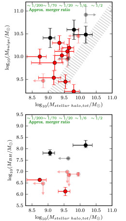
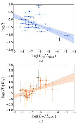
Bulge mass (top) and BH mass (bottom) as a function of stellar halo mass. Red denotes galaxies with low-mass pseudobulges, black shows galaxies with higher-mass classical bulges. The grey shaded area in the bottom plot shows what would be expected if there were a 1:1 correlation between bulge mass and stellar halo mass. [Bell et al. 2017]
Halos as Historical Record
Stellar halos offer a useful way of tracking the merger history of a galaxy. It’s believed that as major mergers with larger satellites occur, a galaxy’s stellar halo will increase in both mass and metallicity as it retains the stars of the satellite.
Bell and collaborators first verify this picture in their sample by plotting the stellar halo metallicities against the stellar halo masses. This check reveals a strong correlation between the two properties that’s consistent with the outcomes from simulations — so the stellar halos indeed encode the merger history of the galaxies. This means that from their halos, we can infer the masses of the largest satellites accreted by these galaxies.
Laboratories for Quiet Accretion
The authors then search for any indication of correlation between the stellar halo mass and the galaxy’s bulge mass or black hole mass. They find that their galaxy sample has a wide range in stellar halo masses that don’t correlate significantly with the bulge-to-total ratio, bulge mass, or black hole mass of the galaxy. This is true not only for the pseudobulges, but also for the classical bulges.
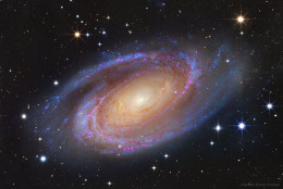
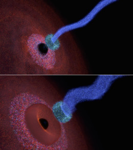
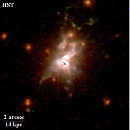
The galaxy M81 has a massive classical bulge but an anemic stellar halo containing only 2% of its total stellar mass. This galaxy may be a useful laboratory for studying quiet accretion events. [Subaru Telescope (NAOJ)/HST/R. Colombari/R. Gendler]
These findings challenge the classical models of massive bulge formation and suggest that more detailed simulations and observations are necessary to unravel how the bulges and black holes at the centers of Milky-Way-like galaxies are grown. In particular, the galaxies with massive classical bulges but without massive stellar halos (the galaxy M81 is suggested as an example) may be ideal laboratories for studying quiet growth mechanisms.
Citation
Eric F. Bell et al 2017 ApJL 837 L8. doi:10.3847/2041-8213/aa6158


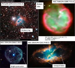
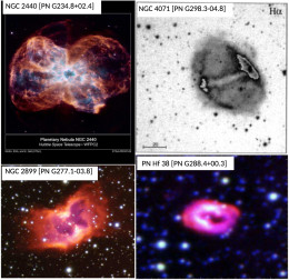
![Examples of planetary nebulae that are extremely likely to have been shaped by a triple stellar system. They have strong departures from asymmetry and don’t show signs of interacting with the interstellar medium. [Bear and Soker 2017]](https://aasnova.org/wp-content/uploads/2017/03/fig2-2-260x292.jpg)

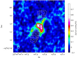
![ALMA observations of the protostar Lupus 3 MMS. The molecular outflows from the protostar are shown in panel a. Panel b shows the continuum emission, which has a compact component that likely traces a disk surrounding the protostar. [Adapted from Yen et al. 2017]](https://aasnova.org/wp-content/uploads/2017/03/fig3-260x529.jpg)


.jpg”)