Where were you on Thursday, 17 August 2017? I was in Idaho, getting ready for Monday morning’s solar eclipse. What I didn’t know was that, at the time, around 70 teams around the world were mobilizing to point their ground- and space-based telescopes at a single patch of sky suspected to host the first gravitational-wave-detected merger of two neutron stars.
Sudden Leaps for Science
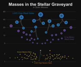
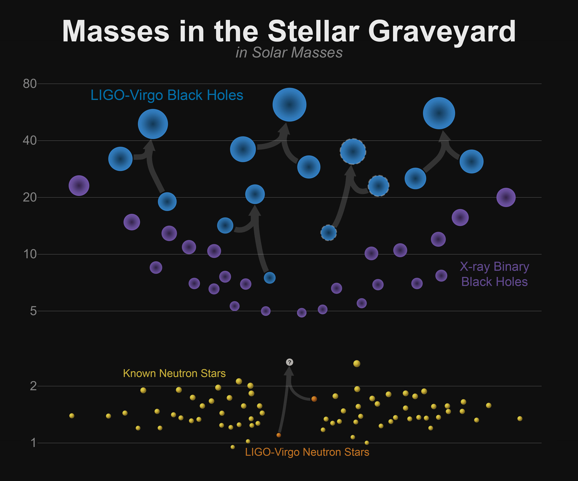
The masses for black holes detected through electromagnetic observations (purple), black holes measured by gravitational-wave observations (blue), neutron stars measured with electromagnetic observations (yellow), and the neutron stars that merged in GW170817 (orange). [LIGO-Virgo/Frank Elavsky/NorthwesternUniversity]
The process of science is long and arduous, generally occurring at a slow plod as theorists make predictions, and observations are then used to chip away at these theories, gradually confirming or disproving them. It is rare that science progresses forward in a giant leap, with years upon years of theories confirmed in one fell swoop.
14 September 2015 marked the day of one such leap, as the Laser Interferometer Gravitational-Wave Observatory (LIGO) detected gravitational waves for the first time — simultaneously verifying that black holes exist, that black-hole binaries exist, and that they can merge on observable timescales, emitting signals that directly confirm the predictions of general relativity.
As it turns out, 17 August 2017 was another such day. On this day, LIGO observed a gravitational-wave signal unlike its previous black-hole detections. Instead, this was a signal consistent with the merger of two neutron stars.
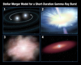
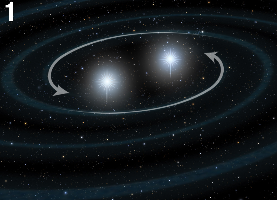
Artist’s illustrations of the stellar-merger model for short gamma-ray bursts. In the model, 1) two neutron stars inspiral, 2) they merge and produce a gamma-ray burst, 3) a small fraction of their mass is flung out and radiates as a kilonova, 4) a massive neutron star or black hole with a disk remains after the event. [NASA, ESA, and A. Feild (STScI)]
What We Predicted
Theoretical models describing the merger of two compact objects predict a chirping gravitational-wave signal as the objects spiral closer and closer. Unlike in a black-hole merger, however, the end of the chirp from merging neutron stars should coincide with a phenomenon known as a short gamma-ray burst: a powerful storm of energetic gamma rays produced as the objects finally collide.
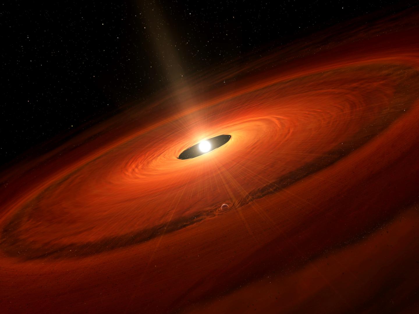
According to the models, these gravitational waves and gamma rays will be followed by a kilonova — a transient source visible in infrared, optical, and ultraviolet — which arises from radioactive decay of heavy elements formed in the collision. This source should gradually decay over a timescale of weeks.
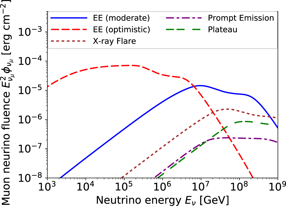
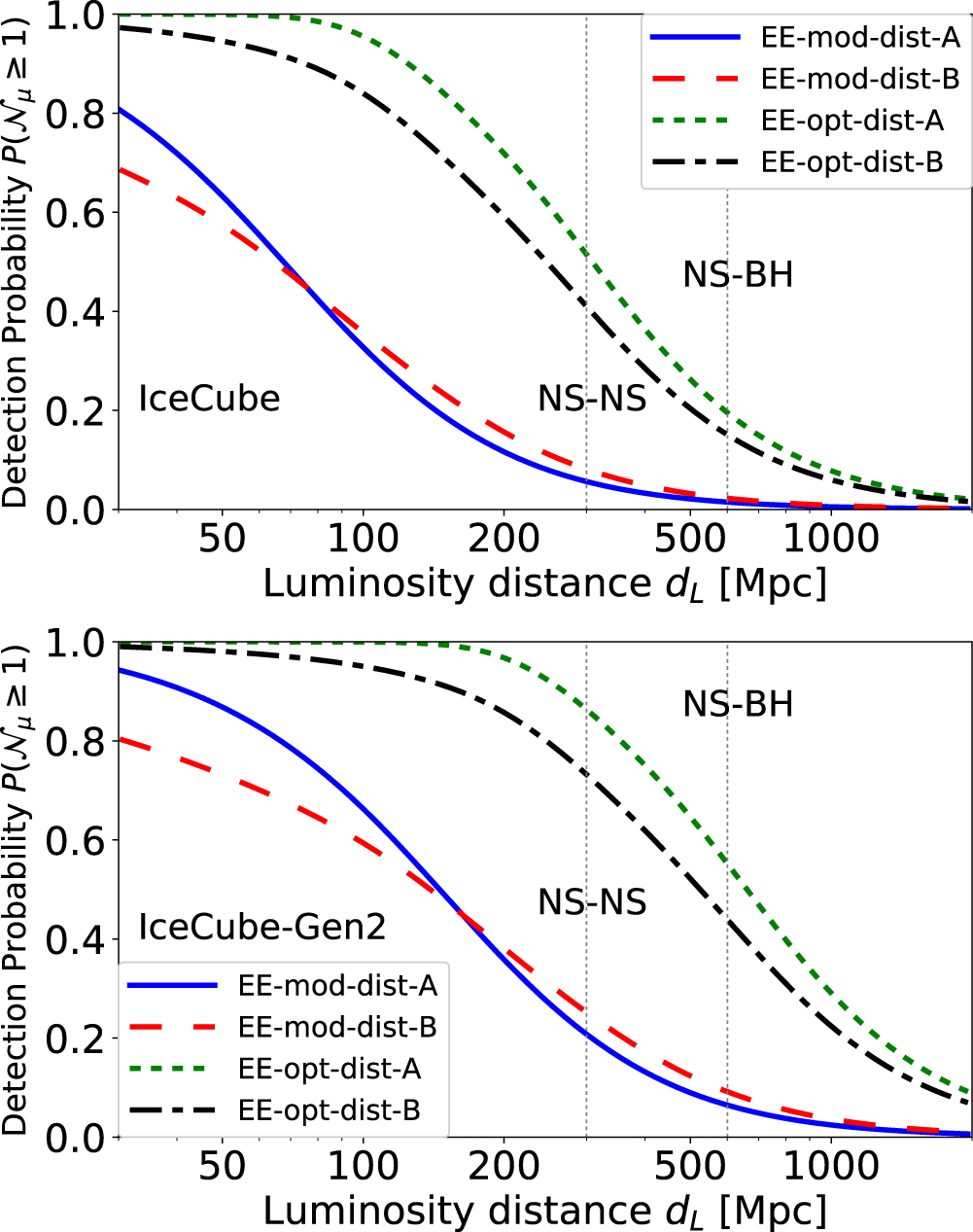
Lastly, the merger could create a powerful jet of high-energy particles, which could be visible to us in X-ray and radio wavelengths as it is emitted and interacts with its surrounding environment. We could also detect neutrinos from this outflow.
What We Saw (and Didn’t See)
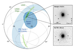
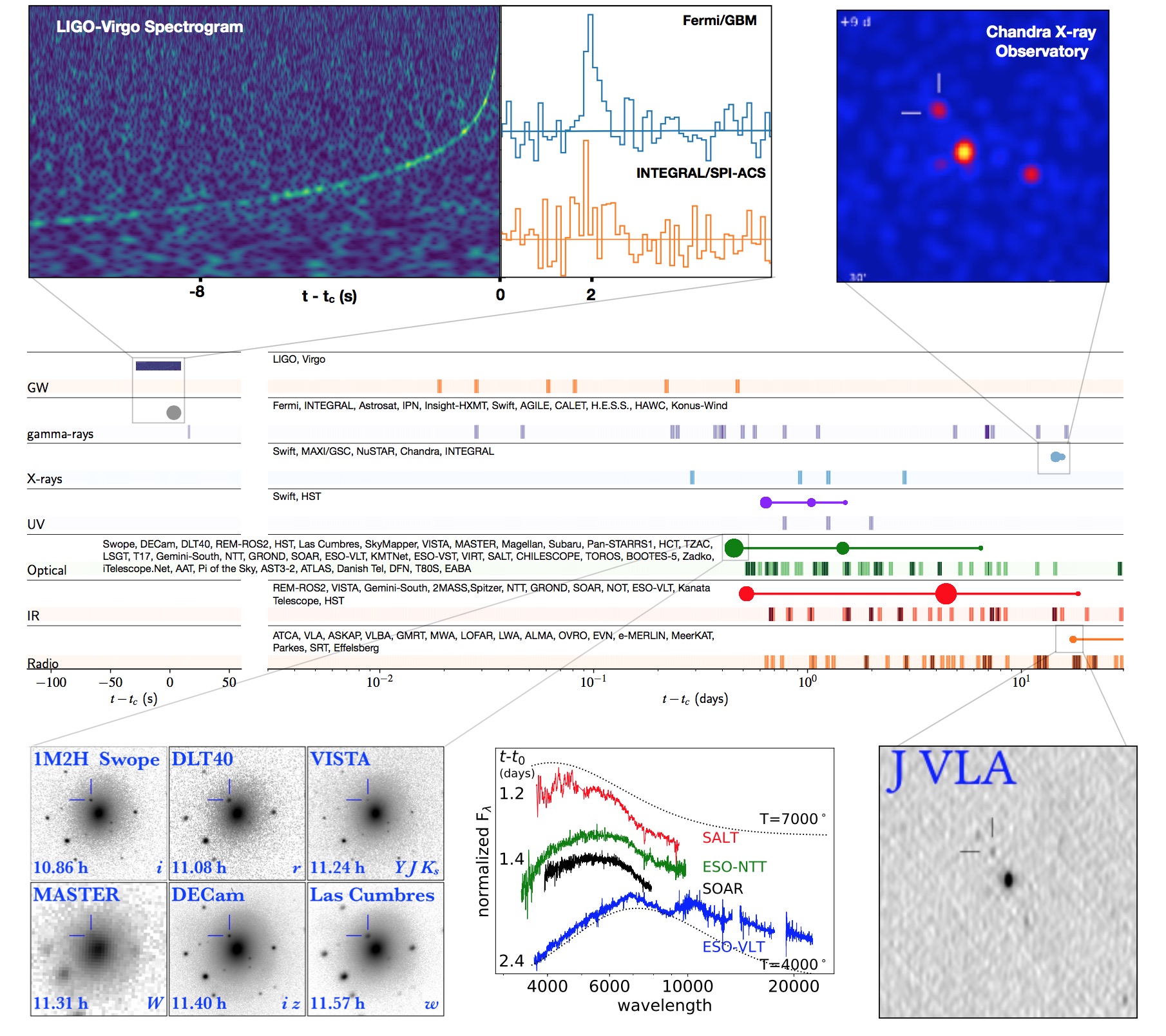
The localization of the gravitational-wave, gamma-ray, and optical signals of the neutron-star merger detected on 17 August, 2017. [Abbott et al. 2017]
So what did we see on 17 August, 2017 and thereafter? Here’s what was found by the army of collaborations searching in gravitational waves, electromagnetic signals across the spectrum, and neutrinos:
- Gravitational Waves
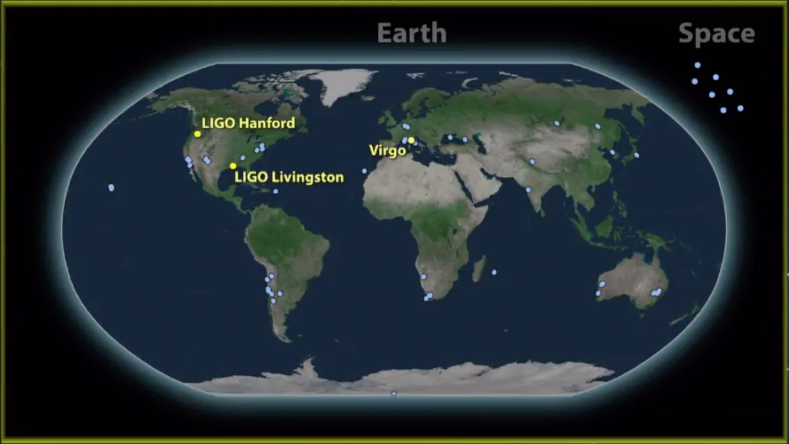
The gravitational-wave signature of a binary neutron-star merger was observed with all three gravitational-wave detectors currently operating as a part of the LIGO-Virgo collaboration. GW170817’s signal was in the sensitivity band of these detectors for ~100 seconds, arriving first at the Virgo detector in Italy, next at LIGO-Livingston in Louisiana 22 milliseconds later, and finally at LIGO-Hanford in Washington 3 milliseconds after that. These detections localized the source to a region of 31 square degrees at a relatively nearby distance of ~130 million light-years, and they identified the binary components to be neutron stars.
- Gamma-Ray Burst
The Fermi Gamma-Ray Burst Monitor detected a short (~2-second) gamma-ray burst, GRB170817A, which appears to have occurred 1.7 seconds after the merger indicated by the gravitational-wave signal. This source was later identified by the International Gamma-Ray Astrophysics Laboratory (INTEGRAL) spacecraft as well.

Locations of the many observatories that observed the neutron-star merger first detected on 17 August, 2017. [Abbott et al. 2017]
Though they were initially foiled by the signal’s location (the localized region of GW170817 only became visible in Chile 10 hours after its detection), the One-Meter, Two-Hemisphere team used the Swope telescope at Las Campanas Observatory in Chile to discover an optical counterpart to the LIGO and Fermi detection, located in the early-type galaxy NGC 4993. Within an hour, five other teams had independently detected the optical source in NGC 4993, with more following after.
In the subsequent hours, days, and weeks, observatories across the electromagnetic spectrum monitored the transient. The source soon faded from view in the ultraviolet and gradually reddened in the optical and infrared bands. Delayed X-ray emission was discovered ~9 days after the LIGO signal, and a radio counterpart was discovered a week after that.- No Neutrinos
Though several neutrino observatories searched for high-energy neutrinos in the direction of NGC 4993 in the two-week period following the merger, none were detected.
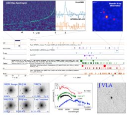
Summary and timeline of the observations of the neutron-star merger detected on 17 August, 2017 relative to the time tc of the gravitational-wave event. Click for a closer look. [Abbott et al. 2017]
A Spectacular Confirmation
So what do these observations tell us? Our model for neutron-star mergers appears to be remarkably successful! The associated detections of gravitational waves and electromagnetic counterparts have confirmed that merging neutron stars produce the expected gravitational-wave signal, that they are the source of gamma-ray bursts, that some of the heaviest elements in the universe are produced during the collision of these stars, and that jets of high-energy particles are created that subsequently interact with their environment.
As with any interesting scientific discovery, new points of exploration have arisen — we can now wonder why the gamma-ray burst was unusually weak given its close distance, for instance, or why we didn’t detect any neutrinos from the outflow.
In spite of our new questions, the combination of these recent discoveries provide a resounding verification of our understanding of how compact objects merge. The various signals that began on 17 August, 2017 have simultaneously confirmed a stack of carefully constructed theories that were crafted over decades to explain how seemingly unrelated electromagnetic signals might all tie together. It’s a beautiful thing when science works out this well!
For more information, check out the ApJL Focus Issue on this result here:
Focus on The Electromagnetic Counterpart of the Neutron Star Binary Merger GW170817
Citation
Abbott, B.P. et al 2017 ApJL 848 L12. doi:10.3847/2041-8213/aa91c9


