
How Do Earth-Sized, Short-Period Planets Form?
Matching theory to observation often requires creative detective work. In a new study, scientists have used a clever test to reveal clues about the birth of speedy, Earth-sized planets.
Former Hot Jupiters?
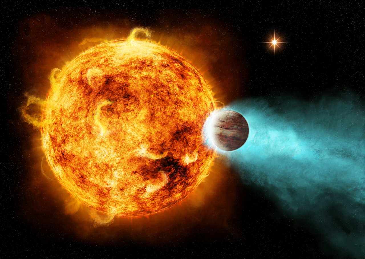
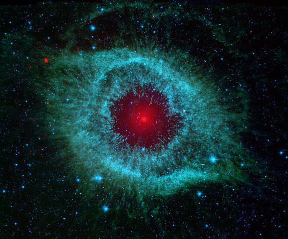
Artist’s impression of a hot Jupiter with an evaporating atmosphere. [NASA/Ames/JPL-Caltech]
How do planets in this odd category form? One popular theory is that they were previously hot Jupiters, especially massive gas giants orbiting very close to their host stars. The close orbit caused the planets’ atmospheres to be stripped away, leaving behind only their dense cores.
In a new study, a team of astronomers led by Joshua Winn (Princeton University) has found a clever way to test this theory.
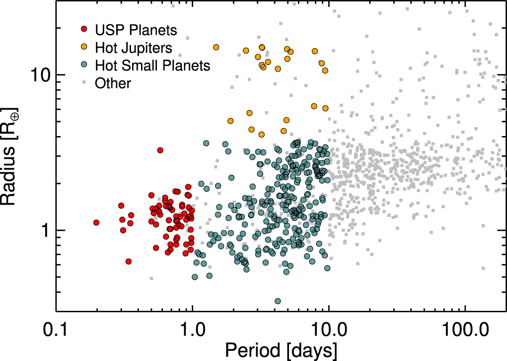
Planetary radius vs. orbital period for the authors’ three statistical samples (colored markers) and the broader sample of stars in the California Kepler Survey. [Winn et al. 2017]
Testing Metallicities
Stars hosting hot Jupiters have an interesting quirk: they typically have metallicities that are significantly higher than an average planet-hosting star. It is speculated that this is because planets are born from the same materials as their host stars, and hot Jupiters require the presence of more metals to be able to form.
Regardless of the cause of this trend, if ultra-short-period planets are in fact the solid cores of former hot Jupiters, then the two categories of planets should have hosts with the same metallicity distributions. The ultra-short-period-planet hosts should therefore also be weighted to higher metallicities than average planet-hosting stars.
To test this, the authors make spectroscopic measurements and gather data for a sample of stellar hosts split into three categories:
- 64 ultra-short-period planets (orbital period shorter than a day)
- 23 hot Jupiters (larger than 4 times Earth’s radius and orbital period shorter than 10 days)
- 243 small hot planets (smaller than 4 times Earth’s radius and orbital period between 1 and 10 days)
They then compare the metallicity distributions of these three groups.
Back to the Drawing Board
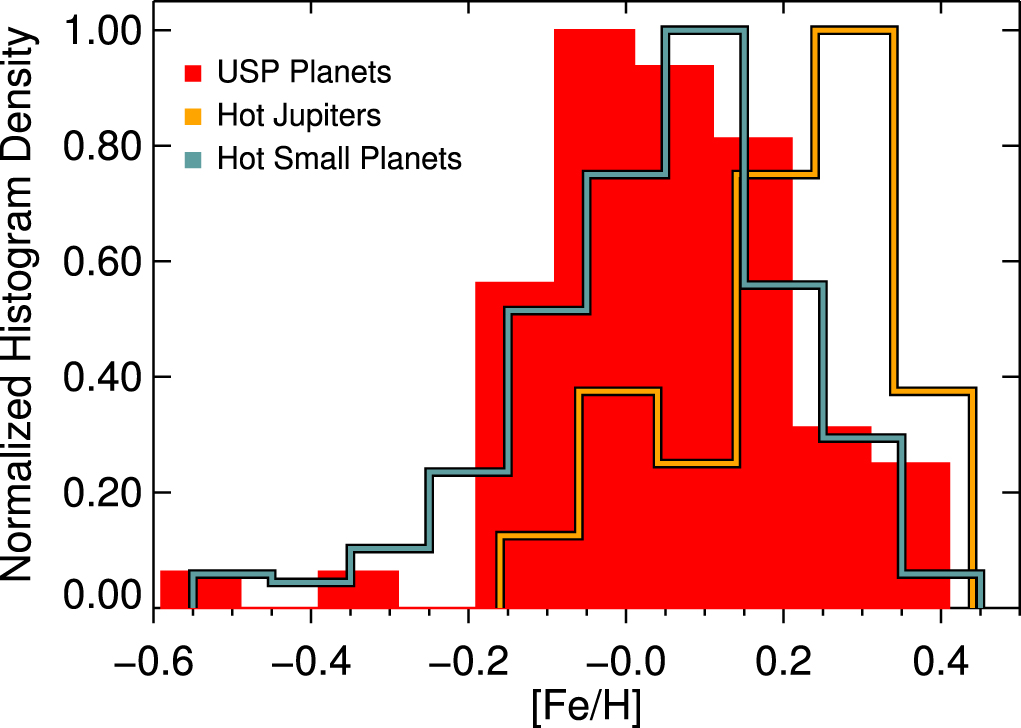
Metallicity distributions of the three statistical samples. The hot-Jupiter hosts (orange) have different distribution than the others; it is weighted more toward higher metallicities. [Winn et al. 2017]
These results strongly suggest that the majority of ultra-short-period planets are not the cores of former hot Jupiters. Alternative options include the possibility that they are the cores of smaller planets, such as sub-Neptunes, or that they are the short-period extension of the distribution of close-in, small rocky planets that formed by core accretion.
This narrowing of the options for the formation of ultra-short-period planets is certainly intriguing. We can hope to further explore possibilities in the future after the Transiting Exoplanet Survey Satellites (TESS) comes online next year; TESS is expected to discover many more ultra-short-period planets that are too faint for Kepler to detect.
Citation
Joshua N. Winn et al 2017 AJ 154 60. doi:10.3847/1538-3881/aa7b7c


