
Piecing Together the Light from Colliding Stars
The recent discovery of GW170817 — the first gravitational-wave detection where we also observed electromagnetic signals — has enabled new studies of merging compact objects. What have we since learned about the radiation that emerges from these collisions?
Signs of a Merger
Before GW170817 was observed, our models predicted that when two compact objects — either two neutron stars, or a neutron star and a black hole — merge, a number of observable signals result:
- a spike of gravitational waves as the objects conclude their death spiral,
- a short gamma-ray burst, an explosion of gamma rays thought to be produced in the relativistic jets launched during the merger,
- an afterglow spanning X-rays to radio, caused when the jets slam into the surrounding environment and decelerate, and
- an optical/near-infrared transient signal called a kilonova, which occurs when neutron-rich ejected material forms heavy elements that then undergo radioactive decay.
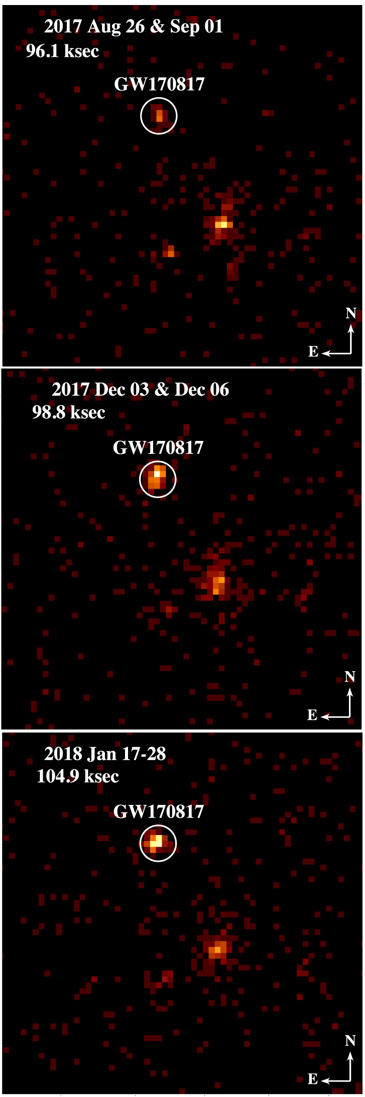
Last August’s binary-neutron-star merger confirmed this picture beautifully: the discovery of gravitational-wave signal GW170817 was followed by detections of short gamma-ray burst SGRB 170817A and later observations of kilonova AT 2017gfo.
But though this was the first time for all of these signals to come together for a source, it wasn’t our first observation of a short gamma-ray burst or a kilonova! How do past detections compare to this new one, and what can we consequently learn about the bursts of radiation from merging compact objects? A team of scientists led by Ben Gompertz (University of Warwick, UK) have now tackled these questions.
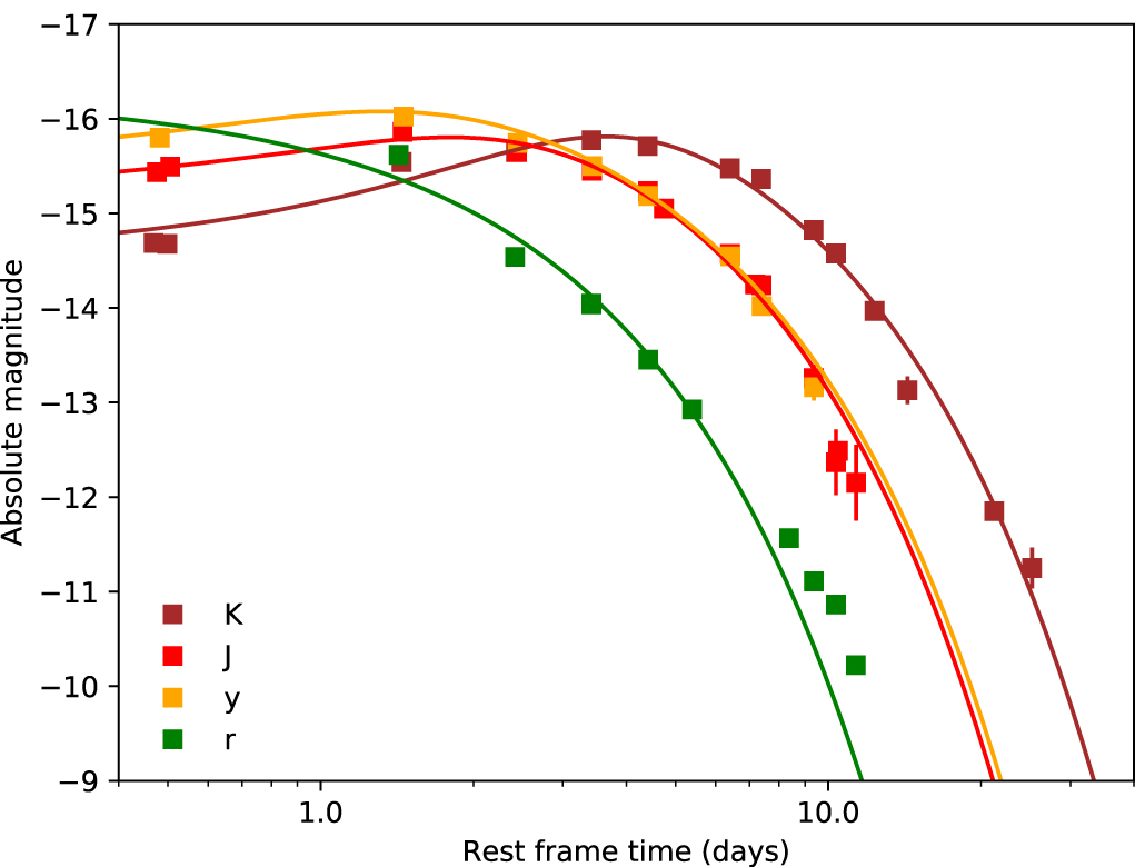
Model fit to the kilonova AT 2017gfo. [Gompertz et al. 2018]
Diversity of Kilonovae
Gompertz and collaborators compared the optical and near-infrared light curves of kilonova AT 2017gfo to equivalent light curves for a sample of a dozen nearby short gamma-ray bursts. What they found was a diversity of signals: some with no evidence of a kilonova, despite observations sensitive enough to pick up a signal several magnitudes fainter than AT 2017gfo; some with confirmed or suspected kilonovae brighter than AT 2017gfo; and some with afterglows so bright that they could be masking kilonovae that are brighter still.
How can we explain these vastly different kilonova outcomes from different mergers? The authors demonstrate that neither line-of-sight dust interference nor viewing angles can explain the differences we see in the optical and near-infrared signals.
It’s All in the Starting Players?
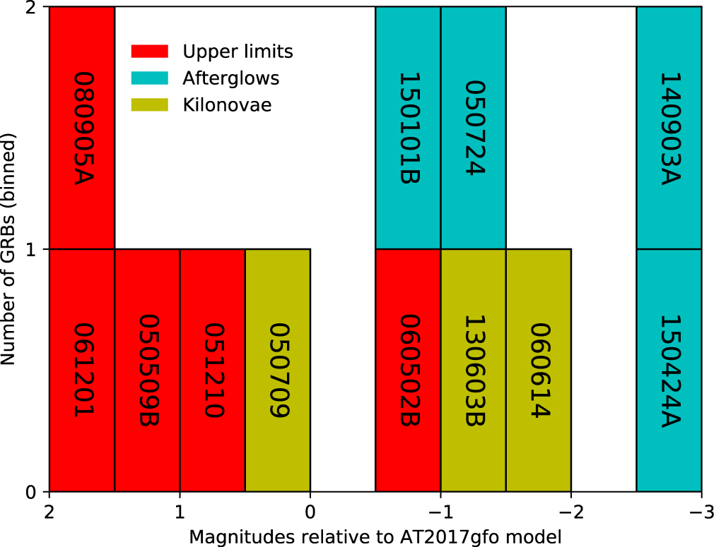
Magnitudes of the optical and near-infrared emission for a sample of 12 short gamma-ray bursts, as compared to the kilonova AT 2017gfo. [Gompertz et al. 2018]
Future observations of these events can confirm or deny this picture, depending on whether the magnitude of kilonova emission continues to display a gap in brightness between two populations, or if it instead forms a continuum. Either way, we can look forward to learning more about these explosive collisions soon!
Citation
B. P. Gompertz et al 2018 ApJ 860 62. doi:10.3847/1538-4357/aac206


