The Origin of Gaps in Protoplanetary Disks
Bright rings and dark gaps are common features in images of protoplanetary disks. How we interpret these features is key to our understanding of how planetary systems form and evolve — so what do these rings and gaps really mean?
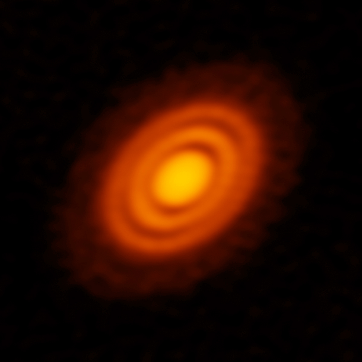
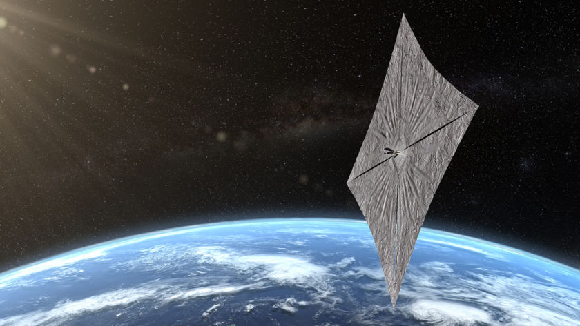
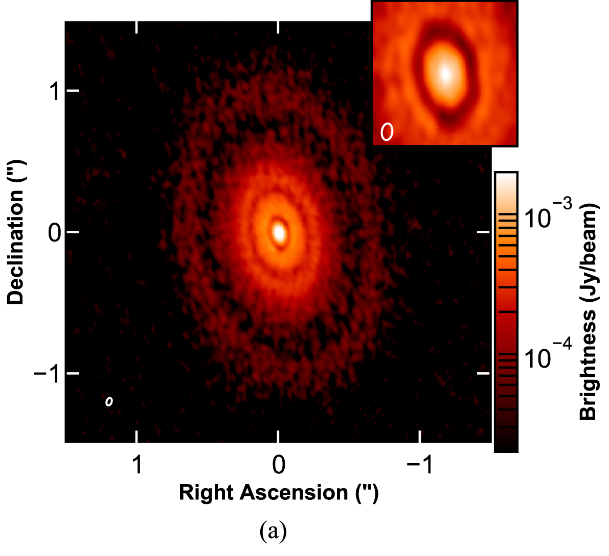
ALMA image of continuum (dust) emission from HD 163296, the subject of today’s paper. [ALMA (ESO/NAOJ/NRAO); A. Isella; B. Saxton (NRAO/AUI/NSF)]
Mind the Gap
The dark lanes that punctuate the bright millimeter emission of protoplanetary disks are often thought to signal the presence of baby planets, which sweep up gas and dust as they orbit their parent star. As exciting as this scenario is, other possibilities exist; the gaps in emission could arise due to gravitational instabilities, the growth of dust grains, or the trapping of dust in high-pressure regions.
How can we distinguish between gaps opened by planets and those generated through other methods? And if the gaps are associated with newly formed planets, how can we reliably extract the properties of the planets — their orbital distances and masses — from the observed gaps in dust emission?
To explore these issues, a team of astronomers led by Nienke van der Marel (National Research Council Herzberg Institute for Astrophysics, Canada) considered the case of the disk surrounding the young star HD 163296.
Interpreting ALMA
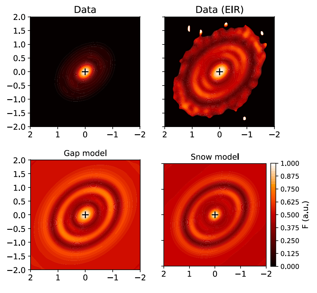
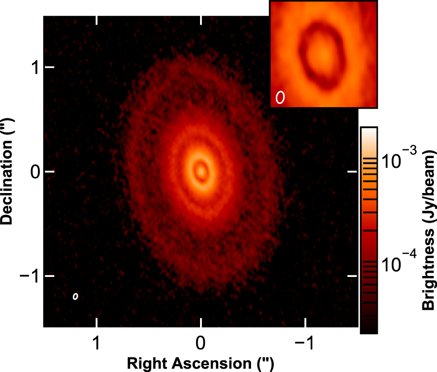
Comparison of ALMA observation of HD 163296 to the same image, enhanced, and the two models. Click to enlarge. [Adapted from van der Marel, Williams & Bruderer 2018]
- The observed gaps in emission are due to a deficit of dust particles inside the gap caused by dust accretion onto a young planet.
- The observed gaps in emission are caused by an increase in the size of the dust grains near snowlines — where it’s cold enough for water, carbon monoxide, and other volatiles to freeze into solids.
Their models show that either planets or snowlines can cause the gaps and rings in the disk around HD 163296. Luckily, we can distinguish between the two scenarios by considering the gas distribution; although the emission is similar in the two models, the presence of planets would decrease both the gas and dust density, whereas the presence of a snowline would not affect the gas density.
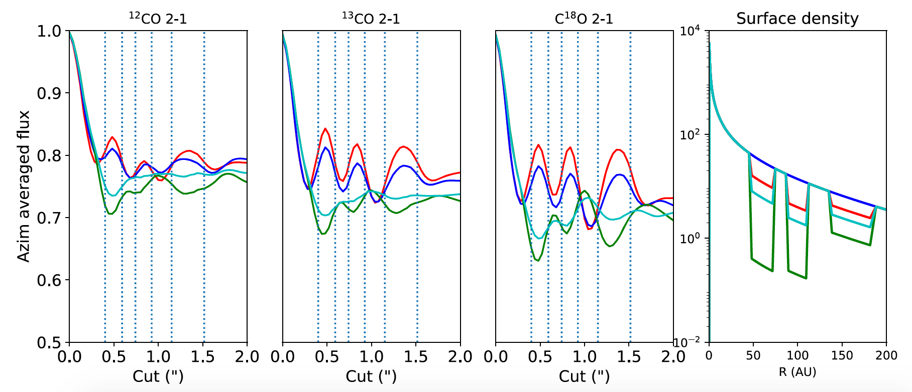
Azimuthally averaged carbon monoxide emission for four modeled gap depths. Shallower gaps correspond to Saturn-mass planets, while deeper gaps correspond to Jupiter-mass planets. Click to enlarge. [van der Marel, Williams & Bruderer 2018]
Taking Cues from Carbon Monoxide
A common tracer of gas in protoplanetary disks is carbon monoxide. When the authors modeled the emission from the carbon monoxide gas, they found something unexpected: as the carbon monoxide density in the gaps decreased, the emission increased.
A closer look at the chemistry reveals why: when gaps are introduced, more of the star’s ultraviolet radiation can reach the gas, which increases its temperature. The increased temperature returns frozen carbon monoxide molecules to the gas phase, which results in increased emission. However, if the gap is sufficiently deep, the warming of the gas isn’t enough to compensate for the decreased density, and the emission decreases.
Because the gap depth is linked to the planet mass, this result underscores the importance of caution when interpreting disk observations. Hopefully, future observations with ALMA can disentangle the roles of planets and snowlines in generating gaps and rings!
Citation
“Rings and Gaps in Protoplanetary Disks: Planets or Snowlines?” Nienke van der Marel, Jonathan P. Williams, and Simon Bruderer 2018 ApJL 867 L14. doi:10.3847/2041-8213/aae88e