The nearby star Regulus — the heart of the constellation Leo — has long been known to be in a binary. But though the bright, main-sequence star is easy to spot, we’ve yet to detect Regulus’s companion! A recent study now presents what may be a first look at this mysterious object.
A Future Entwined
If you’re a star in a close binary system, your fate is not your own. Instead, your future is heavily dependent on how you interact with your companion — especially as you both age.

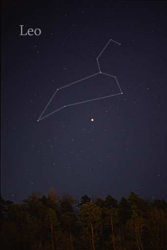
Regulus is the brightest star in the constellation Leo, visible as the star in the lower right corner of the constellation. The bright object below Leo in this photo is Jupiter. [Till Credner; CC BY 3.0]
Such is likely the case for Regulus, a star just ~80 light-years away. Once thought to be a single star, this bright, blue-white, rapidly rotating main-sequence star has since been shown to wobble — it dances in a 40-day orbit with a too-dim-to-spot partner.
May I Have This Dance?
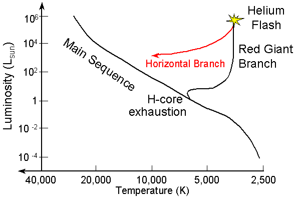
The dance of an interacting, evolving binary is complex. As the more massive star in the pair ages into the red giant stage, it grows larger in size. Eventually, its radius becomes comparable to the separation between it and its less massive, main-sequence partner. At this point, mass and angular momentum begins siphoning off of the massive star onto its main-sequence partner.
As mass and angular momentum continue to transfer, the orbit of the binary first shrinks, and then expands again. At the end of the transfer, the main-sequence star is now bright and rapidly rotating, and the originally massive star has become nothing more than a faint, stripped-down stellar core.
Evidence suggests that this stellar dance is exactly what has happened with Regulus and its undetected companion— but an observational detection of its dim partner would cement this picture. Now, in a study led by Douglas Gies (Georgia State University), a team of scientists may finally have come up with this proof.
Missing Partner Found
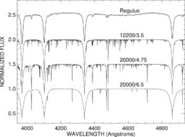
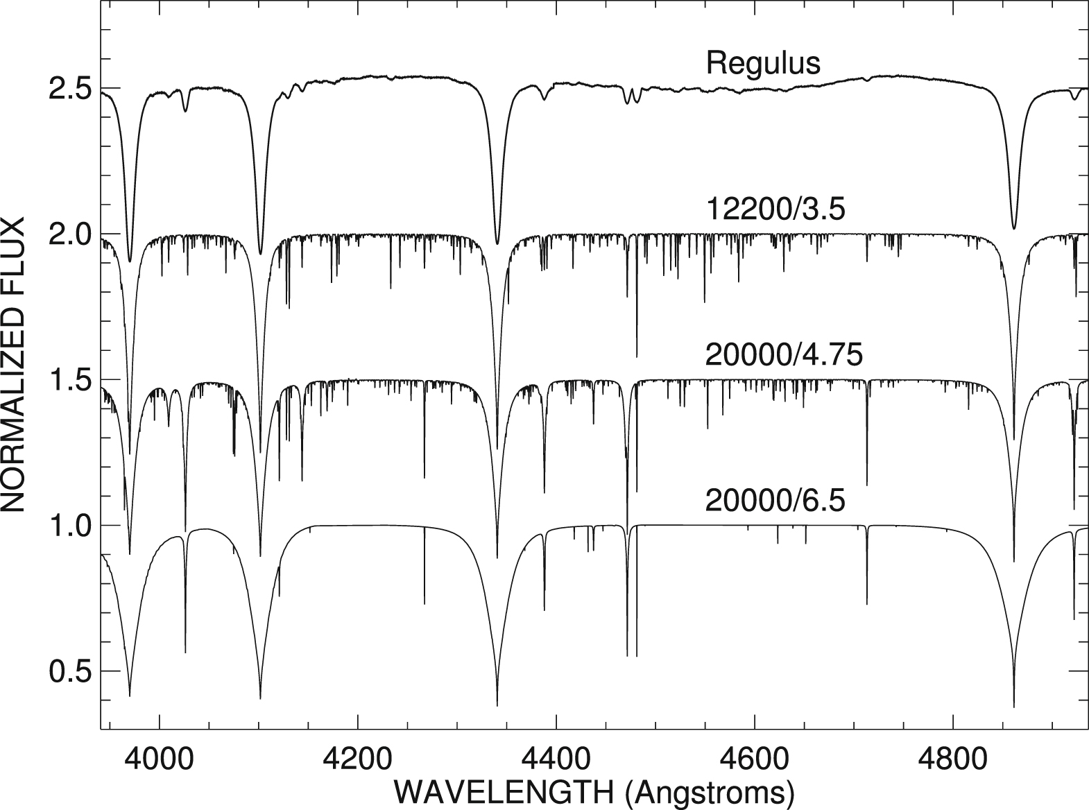
Mean, normalized spectrum of Regulus (generated from 786 CFHT/EsPaDOnS and TBL/NARVAL spectra). Below it are three model spectra used for cross-correlation analysis. [Gies et al. 2020]
Gies and collaborators used the high resolution and high signal-to-noise ratio of the
CFHT/EsPaDOnS and
TBL/NARVAL spectrographs in Hawaii and France to search for the spectral features of Regulus’s dim companion. Though this object is too faint to detect in individual spectra, the authors combine the information from a large set of spectra, use clever cross-correlation analysis to tease out the signature of the weak signal.
Their analysis paid off: Gies and collaborators’ work revealed weak spectral features that have all the properties expected for the spectral signature of the stripped-down companion of Regulus.
The authors find that this surviving core is tiny — just 0.31 solar mass, compared to the Regulus’s 3.7 solar masses — and scalding hot, at perhaps 20,000 K (35,500 °F)! This stripped core will eventually cool and become a white dwarf star.
Regulus and its faint partner confirm our understanding of how stars in a close binary influence each others’ fate. What’s more, the properties of this pair suggest that there may be many, many cases of faint white dwarfs and their progenitors orbiting around bright, rapidly rotating stars.
Citation
“Spectroscopic Detection of the Pre-White Dwarf Companion of Regulus,” Douglas R. Gies et al 2020 ApJ 902 25. doi:10.3847/1538-4357/abb372


