Features RSS

black hole accretion

In April of this year, the Event Horizon Telescope captured the first detailed images of the shadow of a black hole. In a new study, a team of scientists has now explored what determines the size and shape of black hole shadows like this one.

M87 EHT image

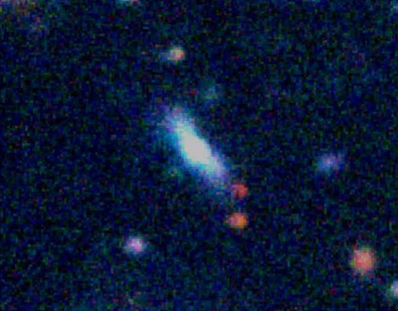
The first detailed image of a black hole, M87, taken with the Event Horizon Telescope. [Adapted from EHT collaboration et al 2019]

Imaging a Shadow

The stunning new radio images of the supermassive black hole in nearby galaxy Messier 87, released this spring by the Event Horizon Telescope team, revealed a bright ring of emission surrounding a dark, circular region.

This distinct structure is a result of the warped spacetime around massive objects like black holes. The ring of light is comprised of photons from the hot, radiating gas that surrounds the black hole, whose paths have been bent around the black hole before arriving at our telescopes. The dark region in the center is termed the black hole’s “shadow”; this is the collection of paths of photons that did not escape, but were instead captured by the black hole.

black hole disk comparison

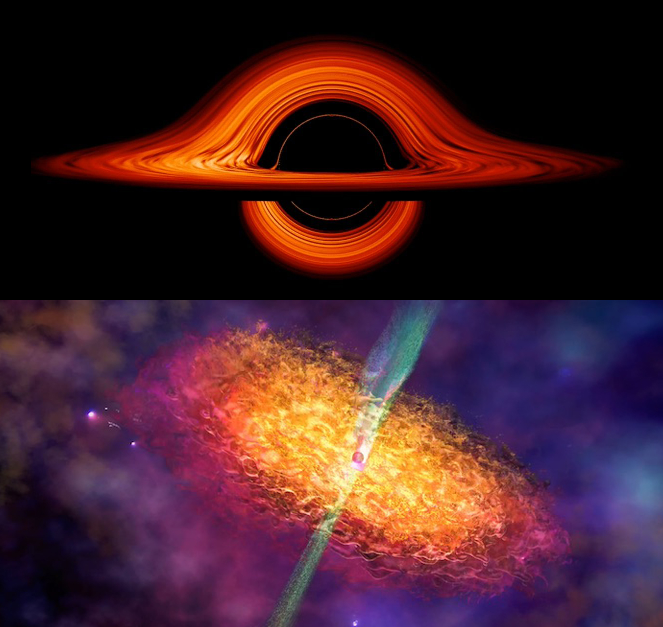
Comparison of conceptions of a black hole surrounded by a thin accretion disk vs. a thick accretion disk. [Top: NASA, bottom: Nicolle R. Fuller/NSF]

The Shape of Accretion

While some previous studies have explored what a black hole shadow looks like when the black hole is surrounded by a very thin disk of accreting gas (think the black hole + disk from the movie Interstellar), most supermassive black holes — like M87, or our own supermassive black hole, Sagittarius A* — are more likely to be surrounded by hot, accreting gas that is more broadly distributed, forming a thick or quasi-spherical disk.

Does the geometry and motion of the accreting gas affect the size and shape of a black hole’s shadow?

Models of Monsters

In a new study, three scientists — Ramesh Narayan and Michael Johnson (Harvard-Smithsonian Center for Astrophysics) and Charles Gammie (University of Illinois at Urbana–Champaign) — have teamed up to explore how a black hole’s shadow changes based on the behavior of the hot gas around it.

black hole shadows

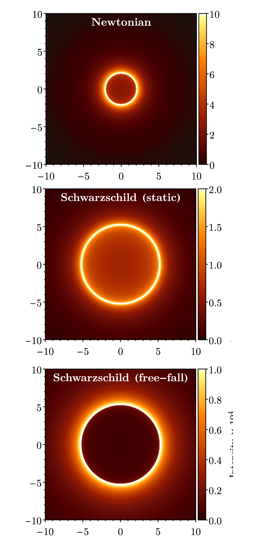
The image of the black hole shadow for three of the authors’ models: non-relativistic spacetime (top), relativistic spacetime with static surrounding gas (center), and relativistic spacetime with accreting gas flowing radially inwards (bottom). [Adapted from Narayan et al. 2019]

Narayan, Johnson, and Gammie built analytical models of a black hole surrounded by hot, optically thin gas (which means that the radiation escapes the gas and is observable). They then analyzed how the shadow would appear using different spacetimes, with different gas motions, and with different behaviors of the gas close to the black hole.

Reducing Complications

Intriguingly, the authors found that the appearance of the black hole’s shadow doesn’t depend on the details of the gas accretion close to the black hole. The size of the shadow was primarily determined by the spacetime itself (which is impacted by the mass of the black hole). But how the gas is distributed around the black hole, and whether that gas is stationary or accreting, doesn’t hugely affect the appearance of the shadow.

Real life is a little messier than this simple, spherically symmetric model; black hole spin and the presence of jets or outflows will cause asymmetries in the shadow. But the authors’ results generally tell us that the close-in details of accretion flows aren’t complicating what we’re seeing. And that’s valuable information we can use as we interpret future observations of black hole shadows! 

Citation

“The Shadow of a Spherically Accreting Black Hole,” Ramesh Narayan et al 2019 ApJL 885 L33. doi:10.3847/2041-8213/ab518c

fast transient

A supernova-like transient was observed to decline stupendously fast. What could have caused it?

Fast Transients

“Fast transients” are objects whose brightness rises and then falls drastically, usually on the order of weeks. They are not regularly varying objects; they have more in common with supernovae, which brighten once and then fade. However, fast transients change more rapidly than supernovae do, suggesting they have different explosive progenitors. 

With the advent of large astronomical surveys, fast transients are spotted more often now than ever before. The “fastest” optical fast transient is kilonova AT2017gfo — the result of the first observed binary neutron star merger. A recent study by Owen McBrien (Queen’s University Belfast) and collaborators discusses a transient that’s right on the heels of AT2017gfo in terms of the speed of its variation: a supernova-like object named SN2018kzr.

Magnetars and Nickel

The host galaxy of SN2018kzr, as seen more than two months after the transient appeared. The image was constructed using data taken by the ESO (European Southern Observatory) Faint Object Spectrograph and Camera on the New Technology Telescope. [Adapted from McBrien et al. 2019]

SN2018kzr was discovered independently by the Zwicky Transient Factory and the Asteroid Terrestrial-impact Last Alert System. Observers were tipped off by its rapid brightening, which took place over hours. SN2018kzr was then observed extensively over the next two weeks by multiple observatories, yielding a wealth of photometric and spectroscopic data. It began declining in brightness the same night it was first detected. 

To explain SN2018kzr’s rise and fall, McBrien and collaborators consider mechanisms that have previously been used for fast transients. They start with the reasonable assumption that nickel-56 is involved. The isotope nickel-56 can form in the explosions associated with fast transients and supernovae, and its radioactive decay can contribute greatly to a transient’s brightness. However, SN2018kzr dims too rapidly for it to be explained by nickel-56 alone, and the decay of other radioactive isotopes don’t explain observations either.

One solution is to tweak the progenitor scenario to include a massive remnant: a rotating neutron star with a strong magnetic field, known as a magnetar. A magnetar can contribute to the energy put out by SN2018kzr by slowing its own rotation. When coupled with nickel-56 decay, a magnetar’s spin-down could explain the shape of SN2018kzr’s light curve.

Choose Your Scenario

Fits to the light curve of SN2018kzr assuming different progenitor scenarios. The red points are associated with SN2018kzr and the white diamonds are associated with another fast transient, SN2005ek. SN2005ek is better fit by the He star model, while SN2018kzr is better fit by the nickel-56–magnetar scenario. [Adapted from McBrien et al. 2019]

Assuming that nickel-56 and a magnetar are involved in the progenitor of SN2018kzr, the authors present three possible scenarios: the core-collapse of a helium-rich star, the collapse of a white dwarf that’s accreted too much matter (accretion induced collapse, or AIC), and the merger of a white dwarf and a neutron star.

The first scenario isn’t favored since any remnant it produces wouldn’t rotate fast enough to explain SN2018kzr’s rapid decline. The authors favor the other scenarios, though the AIC model is on shaky ground based on previous studies.

The more fast transients we discover, the better our understanding becomes of how they form. Stay tuned!

Citation

“SN2018kzr: a rapidly declining transient from the destruction of a white dwarf,” Owen R. McBrien et al 2019 ApJL 885 L23. https://doi.org/10.3847/2041-8213/ab4dae

solar magnetic field

General models of the Sun’s atmosphere have a fundamental problem: the magnetic flux they predict here at Earth is much lower than what we actually observe. Has a new study found the missing flux?

When Models and Observations Don’t Match

The Sun offers us a unique opportunity to study stellar magnetic fields up close, testing the match-up between our models and observations — but, unfortunately, the outcome isn’t always ideal.

Sun's magnetic field lines

Magnetic field lines drawn from the solar surface to two times the Sun’s radius. The Sun’s magnetic field permeates our solar system as an interplanetary magnetic field. [Adapted from Riley et al. 2019]

Global models of the Sun’s atmosphere match the observed magnetic fields at its photosphere (the solar surface), and they do a great job of reproducing many features of the corona (the Sun’s extended upper atmosphere) and the solar wind (the stream of energetic particles that flows from the Sun into interplanetary space).

The trouble comes when we take a closer look at the predicted strength of the modeled interplanetary magnetic field — the natural extension of the solar magnetic field into the solar system. It’s there that our global solar models have a problem: they often underpredict the strength of the interplanetary magnetic field at a distance of 1 AU (i.e., at Earth, where we can easily measure it) by a factor of two or more.

So where’s the missing magnetic flux?

solar magnetic field

Line-of-sight component of the solar magnetic field, mapped out for models without (top row) and with (bottom row) extra flux added at the poles, as seen from two different vantage points: the view from Earth in the Sun’s equatorial plane (left column), and the view from a point 30° above the equatorial plane (right column). From Earth the difference is not visible; from 30° above, it will be. [Adapted from Riley et al. 2019]

Adding to the Poles

Led by Pete Riley, a team of scientists at Predictive Science Inc. in San Diego have proposed a solution: what if this “missing” flux takes the form of concentrated bundles of magnetic flux at the solar poles that we just can’t see from our angle?

Earth’s position near the plane of the Sun’s equator makes it difficult for us to observe much of what’s happening at its poles. It’s entirely possible that there’s extra magnetic flux at the poles of the Sun — where we can’t resolve it with ground-based observatories or Earth-based spacecraft — that our models are missing. By adding this flux into our models, maybe we’ll be able to reproduce the interplanetary magnetic field measured at Earth.

A Better View Ahead

To test this theory, Riley and collaborators explore a series of global models of the Sun, reconstructing the coronal magnetic field and measuring the resulting magnetic flux at 1 AU. In their models, the authors add extra bundles of open magnetic field lines at the poles of the Sun, and they then test whether this addition creates any other changes that would conflict with current solar observations.

Solar Orbiter

Artist’s impression of the ESA/NASA Solar Orbiter mission. [ESA/C. Carreau]

The authors find that their added flux significantly reduces the problem of the underpredicted interplanetary magnetic field — their values are much closer to the measured values. What’s more, the added flux also doesn’t produce any new observational discrepancies; the authors’ models still produce features in the corona consistent with what we see (and in some cases, even provide a better reproduction of observations).

So how can we tell if this is a realistic solution? The upcoming joint ESA/NASA Solar Orbiter mission, launching in February 2020, is just what we need: this spacecraft will eventually orbit the Sun at an inclination of 25° and above, allowing us a more definitive look at the Sun’s poles.

Citation

“Can an Unobserved Concentration of Magnetic Flux Above the Poles of the Sun Resolve the Open Flux Problem?,” Pete Riley et al 2019 ApJ 884 18. doi:10.3847/1538-4357/ab3a98

giant collision

How do you get close-in, giant planets on eccentric orbits? A new study suggests that a violent phase of planet-smashing might be a key part of the process.

High-Mass Lurkers

hot Jupiter

Artist’s impression of a close-in, giant exoplanet transiting across the face of its host star. [NASA/ESA/C. Carreau]

In our ever-growing tally of observed exoplanets (we’re up to 4093 confirmed now!), there are several intriguing categories of planets that have no analog in our own solar system. Looming large among these are close-in gas giants.

We’ve discovered quite a few gas giants that have orbital distances of less than 5 AU from their host stars, and the orbits of these planets are often eccentric — making them very unlike the well-behaved, nearly circular orbits of the planets in our solar system.

What causes the eccentricities of these giants? Numerous mechanisms have been proposed, from complex gravitational interactions between the inner giant planets and outer companions, to resonant interactions with a gas disk early in the stellar system’s formation.

But in a recent study led by Renata Frelikh (UCO/Lick Observatory, UC Santa Cruz), a team of scientists has explored a more dramatic scenario: what if eccentric, close-in giant planets are the result of a period of giant impacts?

Giant impact

Artist’s concept of two bodies colliding during the early stages of planet formation. [NASA/JPL-Caltech]

Coming Together Through Collisions

One of the leading theories for the formation of our own solar system predicts that, at the end of the assembly period for the inner solar system, our system underwent a giant-impact phase. During this time, hot young planetesimals smashed into one another — in fact, one of these collisions is blamed for throwing off material from Earth to later form the Moon.

Frelikh and collaborators propose that when planetary systems hosting multiple hydrogen-rich planets in their inner regions undergo a similar giant-impact phase, collisions can cause these planets to grow in mass as they merge. The collisions and scatterings eventually produce large, gaseous planets on close-in, eccentric orbits.

To test their theory, the authors conduct a series of N-body simulations tracking the collisions and mergers of planets in the inner regions of a modeled planetary system. They then compare their results to the properties of an observed sample of exoplanets orbiting F, G, and K stars.

More Mass, More Giants

eccentricity vs. mass

Plots of eccentricity vs. mass as an example comparison of the distributions for observed planets (top panel) vs. authors’ simulated data (bottom panel). [Adapted from Frelikh et al. 2019]

Frelikh and collaborators find that high-eccentricity giants like those we observe today appear to form preferentially in systems that start with a higher initial total planet mass in the inner disk — regardless of whether that initial mass is distributed in the form of a few large planets or lots of small planets at the start of the simulation.

They demonstrate that planet–planet collisions and scattering in their simulations leads to a distribution of eccentricities, orbit sizes, and planet masses at the end of the giant-impact phase that are consistent with the sample of planets we’ve observed.

The predictions made by the authors’ models can be tested further as we build a larger sample of observed exoplanets both in stellar systems’ inner and outer regions. But for now, this provides new insight into the potentially violent pasts of some of the unusual planets we’ve discovered.

Citation

“Signatures of a Planet–Planet Impacts Phase in Exoplanetary Systems Hosting Giant Planets,” Renata Frelikh et al 2019 ApJL 884 L47. doi:10.3847/2041-8213/ab4a7b

Large Magellanic Cloud

As the Large Magellanic Cloud plows through the Milky Way’s dark matter halo, it may leave telltale signs of its passage. A recent study explores whether we’ll be able to spot this evidence — and what it can tell us about our galaxy and the nature of dark matter.

The Milky Way’s Large Companion

LMC and SMC

The Large and Small Magellanic clouds, as observed from Earth. [ESO/S. Brunier]

The Milky Way is far from lonely. Dozens of smaller satellite-galaxy companions orbit around our galaxy, charging through its larger dark matter halo. The most massive of these is the Large Magellanic Cloud (LMC), a galaxy of perhaps 10 or 100 billion solar masses that’s about 14,000 light-years across.

Studies suggest that the LMC is on its first pass around the Milky Way, traveling on a highly eccentric orbit; it likely only first got close to our galaxy (within about 200 kpc, or 650,000 light-years) about two billion years ago.

There are still many uncertainties about this satellite and its travels, however. How massive, exactly, is the LMC? What does its past orbit look like? And how has it interacted with our galaxy’s dark matter halo, which it’s passing through? 

LMC wake

Density perturbations caused by the LMC’s motion for one of the authors’ Milky Way models. The Milky Way’s disk is in the x–y plane; the black curve traces the LMC’s past orbital path and the red star indicates its current position. Three primary overdense/underdense features are visible as signatures of the LMC’s wake. [Adapted from Garavito-Camargo et al. 2019]

A Telltale Trail

A team of scientists led by Nicolas Garavito-Camargo (Steward Observatory, University of Arizona) thinks there may be evidence we can use to answer these questions.

Like a boat, the LMC should generate a wake as it plows through the Milky Way’s dark matter halo. This wake is caused by gravitational interactions between the satellite and dark matter particles that drag at the LMC, causing the galaxy to lose angular momentum as it orbits.

The perturbations that make up this wake — overdensities and underdensities in the dark matter and stellar distribution in the halo — are signatures that we can predict and hunt for. In a new study, Garavito-Camargo and collaborators use high-resolution N-body simulations to explore the motion of the LMC through the Milky Way’s halo and examine the perturbations caused by this charging satellite.

Spotting the Evidence of Passage

The authors find that the LMC’s motion produces a pronounced dark matter wake that can be decomposed into three parts:

  1. Transient response, a trailing wake of overdensity behind the satellite that traces its orbital history
  2. Global underdensity, a large underdense region south of the transient response
  3. Collective response, an extended overdensity leading the LMC in the galactic north

These features in the dark-matter distribution are echoed in how stars are distributed in the regions, and the stars should also show distinctive kinematic signatures.

observing strategy

Observing strategies for identifying the LMC’s wake using stellar densities. To avoid confusion with the Sagittarius stellar stream (the prominent yellow, orange, and red points indicated), the authors identify several regions for observation (colored rectangles) away from the stream where the wake should be detectable. Click to enlarge. [Garavito-Camargo et al. 2019]

Garavito-Camargo and collaborators outline an observing strategy to spot the predicted overdensities and underdensities of the wake, and they show that the detection of just 20–30 stars in specific regions could provide useful confirmation of their models. The measurements needed should be achievable with current and upcoming stellar surveys.

What can we learn from these observations? The detection of the LMC’s wake will track its past orbit, which will provide an indirect measure of our own galaxy’s mass. The specifics of the LMC’s motion will also better constrain the satellite’s mass, as well as provide clues as to the nature of the dark-matter particles that drag on it.

Citation

“Hunting for the Dark Matter Wake Induced by the Large Magellanic Cloud,” Nicolas Garavito-Camargo et al 2019 ApJ 884 51. doi:10.3847/1538-4357/ab32eb

Crab nebula

The same physical phenomenon that causes bumpy airplane rides also pervades our universe, jumbling stellar atmospheres, interstellar clouds, and even the magnetized sheath surrounding the Earth. Now, a new study brings us a little closer to understanding turbulence.

turbulence

This image captures the transition between laminar and turbulent flow in the convection plume above a candle flame. [Gary Settles]

A Complex Phenomenon

Have you ever watched the entrancing wisps of smoke rising above a candle flame? What you’re looking at is turbulence — and despite this phenomenon’s prevalence throughout the universe, a complete description of turbulence remains one of the unsolved problems in physics.

The difficulty is that turbulent motion — characterized by rapid and chaotic fluctuations of fluid properties — is incredibly complex. Turbulence begins when energy is injected on large scales, causing field-level fluctuations. This energy then cascades down to smaller and smaller scales, creating chaotic motions all the way down to microscales. When the energy reaches small enough scales, it can dissipate, accelerating individual particles and converting into heat.

But scientists don’t fully understand the physical mechanisms at work in turbulence that inject the energy, transfer it to smaller scales, and eventually dissipate it. Worse yet, these processes take a different form when we’re no longer talking about fluids, but instead about astrophysical plasmas.

Plasmas, Plasmas Everywhere

Astrophysical plasmas are soups of ionized gas found everywhere from supernova remnants to the compressed solar wind surrounding the Earth in its magnetosheath — and in these plasmas, energy could be dissipated through a variety of mechanisms related to interactions between particles and waves.

magnetosphere

This diagram of the Earth’s magnetosphere shows the location of the magnetosheath, the region behind the bow shock where the compressed solar wind detours around the Earth. [NASA/Goddard/Aaron Kaase]

How can we tell which mechanisms are at work? The key is to explore the rate at which turbulence in a plasma is dissipated across different length scales. In a recent study, a team of scientists led by Jiansen He (Peking University, China) has now developed a new approach to examine this spectrum and applied it within the Earth’s magnetosheath.

Measuring a Fluctuating Environment

The authors’ approach takes advantage of unprecedented, high-quality measurements made by the Magnetospheric Multiscale mission, a constellation of four spacecraft exploring the plasma environment around the Earth. As these spacecraft — separated by a distance of about 10 km — pass through magnetosheath plasma, they make measurements of the three-dimensional electric and magnetic fields, tracking the field fluctuations caused by turbulence.

MMS

Artist depiction of the Magnetospheric Multiscale Mission spacecraft. [NASA/GSFC]

He and collaborators present a method that uses these measured fluctuations to investigate how the dissipation rate is distributed across various length scales within the plasma. This spectrum of dissipation rates can then tell us which physical processes are most likely at play, driving the dissipation.

While we still have a lot to learn, He and collaborators’ work indicates that ion cyclotron waves — waves generated when ions oscillate in a magnetized plasma — play an important role in dissipating turbulent energy in the Earth’s magnetosheath.

More importantly, the authors’ approach for measuring the dissipation rates at different scales can be widely applied to different space plasma environments — so we can hope for more insight into turbulence in space in the future!

Citation

“Direct Measurement of the Dissipation Rate Spectrum around Ion Kinetic Scales in Space Plasma Turbulence,” Jiansen He et al 2019 ApJ 880 121. doi:10.3847/1538-4357/ab2a79

Being able to make precise measurements of distances and redshifts will help us understand how the universe is evolving. With the advent of gravitational wave observatories, we can make these measurements by using black holes in a very different way than before.

Standard Sirens

To measure how the universe is expanding, we need to simultaneously obtain the distances and redshifts to sources. When it comes to measuring large distances in space, astronomers have typically leaned on “standard candles” — objects whose intrinsic brightness is known. The dimmer a standard candle appears, the farther away it is.

Merging binary black holes (BBHs) can serve as standard candles, in a way. When compact objects like black holes merge, they produce gravitational waves, which can be picked up by observatories like the Laser Interferometer Gravitational-Wave Observatory (LIGO). The emitted gravitational waves have a characteristic energy, meaning that these mergers could be used to measure distances as “standard sirens”.

The trouble comes when trying to simultaneously measure the redshift of these sources. The gravitational wave detection on Earth gives us a mass measurement for the black holes that’s a combination of their redshift and their true masses in the source frame. If we know the true masses, we can disentangle these variables and determine the redshift. To achieve this, Will Farr (Stony Brook University and Flatiron Institute) and collaborators propose using a particular constraint on the masses of BBHs.

True black hole mass (not measured mass) versus redshift as obtained from one year of simulated BBH merger observations. The blue line indicates the maximum mass of black holes as set by PISNs, with the dark and light bars showing the confidence intervals. [Farr et al. 2019]

Capping Masses

When we model the population of merging black holes we’ve detected via gravitational wave observations, we see a drop-off in black hole mass above 45 solar masses. Farr and collaborators suggest this upper limit could be tied to one specific route of black hole creation: pair instability supernovae (PISNs).

Only massive stars can die as PISNs. In these events, the core of a star gets hot enough to allow electron–positron pairs to pop into existence, which lowers the star’s internal pressure enough for gravity to trigger the trademark explosion of a supernova. The remnants left behind by PISNs peak in mass around 45 solar masses. 

By taking advantage of the mass scale imprinted on the population of BBH mergers by the PISN process, Farr and collaborators argue, we can extract redshifts from our detector measurements. Simulating 5 years of detections, the authors show that we could potentially constrain the Hubble parameter — our measurement of the expansion of the universe — at a specific redshift to within an impressive 2.9%.

Distributions of the Hubble parameter at a redshift of 0.8 as estimated by one year of observations (blue) and five years of observations (orange). The true value of the Hubble parameter at that redshift is indicated by the black vertical line. [Adapted from Farr et al. 2019]

Paring Down Parameters

The authors find that BBHs are most useful for constraining the Hubble parameter at a redshift of z = 0.8 (redshifts that can be explored with the current capabilities of gravitational wave observatories are between = 0 and 1.5). This is because at that redshift the models peg the uncertainty on the Hubble parameter at a minimum. Additionally, the uncertainty is halved when going from one year of observations to five years.

The authors note that a change of 1–2 solar masses in their maximum black hole mass does not change their results drastically. Their method would also work with a different maximum mass — so long as there is some mass scale, BBH mergers can be used to measure distances.

New gravitational-wave detectors will extend our sample of BBH mergers enormously. With a larger sample and a better understanding of the utility of black holes, we will be closer to pinning down the fate of the universe.

Citation

“A Future Percent-level Measurement of the Hubble Expansion at Redshift 0.8 with Advanced LIGO,” Will M. Farr et al 2019 ApJL 883 L42. https://doi.org/10.3847/2041-8213/ab4284

exoplanet system

Though we’ve discovered thousands of planets beyond our solar system, we still have a lot to learn about how these bodies form and evolve. Now, a newly discovered baby planetary system may provide some insight.

Multiplanet Wealth

Kepler systems

An illustration of some of the planetary systems discovered by the Kepler spacecraft. The stars at the centers of these systems are not pictured. [NASA Ames/UC Santa Cruz]

The Kepler mission has been instrumental in our exploration of worlds beyond our solar system, helping us to discover nearly 5,000 confirmed and candidate exoplanets. In particular, Kepler’s gaze has revealed a wealth of compact, multiplanet systems that share both intriguing similarities and striking differences with our own solar system.

Kepler multiplanet systems tend to be coplanar, with nearly circular orbits and low obliquities. There is often a high degree of intrasystem uniformity — planets of similar sizes, masses, and orbital spacing are more likely to be found together in the same system. And, intriguingly, most Kepler compact multiplanet systems tend to consist of small planets that have radii of less than 3 Earth radii.

Could these systems’ traits point to how they form and evolve? Might these planets once have had larger sizes, before they cooled and contracted or lost some of their atmospheres to photoevaporation? In order to answer these questions, we need to explore multiplanet systems much earlier in their lifetimes.

V1298 Tau transit light curves

Phase-folded transits for each of the four V1298 Tau planet candidates. [Adapted from David et al. 2019]

New Baby Planets Found

Now, a team of scientists led by Trevor David (Jet Propulsion Laboratory, California Institute of Technology) has identified a system of planets that might be exactly what we’re looking for.

David and collaborators re-analyzed Kepler data from 2015 to identify three new planets transiting the young solar analog V1298 Tau, which was already known to host one Jupiter-sized planet on a 24 day orbit. The newly discovered planets have periods of 8.25 days, 12.46 days, and somewhere between 36 and 223 days (we only have one transit for this last one, so its orbit isn’t yet well-constrained).

Critically, V1298 Tau is a very young star, at just 23 million years old — so we’re examining this planetary system early in its formation.

A Valuable Laboratory

Young transiting exoplanets

Young transiting exoplanets in the period–radius plane. The new planets discovered around V1298 Tau are indicated by yellow stars, and they occupy sparsely populated regions of the plane. Click to enlarge. [David et al. 2019]

What makes the planets of the V1298 Tau system interesting is their unusually large sizes: though their masses are low, these planets are Neptune-to-Saturn-sized, clocking in at 5.6, 6.4, and 8.7 Earth radii. V1298 Tau’s planets are therefore significantly larger than the planets found in the vast majority of Kepler multiplanet systems.

The authors speculate that these planets may still be radiatively cooling and contracting, and perhaps losing atmosphere. The V1298 Tau system could, in fact, be the precursor to the compact multiplanet systems Kepler has found throughout the galaxy.

V1298 Tau provides a valuable laboratory to explore a stellar system in the early stages of its evolution. By following up with additional observations — such as planet mass measurements and atmospheric characterization — we stand to learn much more about how this baby planetary system and others like it formed and evolved.

Citation

“Four Newborn Planets Transiting the Young Solar Analog V1298 Tau,” Trevor J. David et al 2019 ApJL 885 L12. doi:10.3847/2041-8213/ab4c99

Kepler-186f

How can we identify life on other planets? The Earth might be able to help with that — specifically with something called the red edge.

The Green Light for Life

One of the most exciting prospects of exoplanet science is discovering another planet that can harbor life. However, this necessitates us knowing how to identify life at a distance, which is quite a challenge!

The light reflected by an exoplanet is one of the most useful observations to have on this quest. The reflected light is dependent on the surface and atmospheric conditions of the planet, and it may hold key features that point to the existence of life. What those features are, however, is another question.

Blue Marble

Photograph of the Earth taken from space. [NASA/Goddard Space Flight Center/Reto Stöckli]

This is where the Earth comes in handy. With our intimate understanding of the Earth, we can simulate it as an exoplanet fairly accurately. Those simulations can help us better pick out Earth-like planets from reflected-light observations.

The Earth’s reflected-light spectrum contains a unique feature: something called the red edge, a region of rapid change in the near-infrared part of the spectrum. The red edge is caused by chlorophyll in the Earth’s organisms, which has the quirk of strongly reflecting red light. Could this red edge be used to identify chlorophyll-containing life on other planets? In a recent study, Jack O’Malley-James and Lisa Kaltenegger (Carl Sagan Institute, Cornell University) considered the effects of various organisms on the red edge and what that means for the red edge’s detectability.

Exploring Scenarios

A surprising number of organisms contain chlorophyll, but at present, land-based vegetation is most responsible for the red edge. Aside from trees (a catchall term for land-based vegetation), O’Malley-James and Kaltenegger considered other organisms like cyanobacteria, algae, and lichens.

Initially, the authors used a simplified model of the Earth to understand the impact of each organism. They assumed that the entirety of the planet was covered by just one organism and determined how the red edge would appear for an atmosphere that was still like the Earth’s. They then tried the same scenario with a more realistic Earth, which had a surface that was 30% land and 70% ocean.

The authors also considered the effect of clouds. They tried two cases for each planet scenario, one with clear skies and the other with 60% cloud cover. The difference in cloud cover was more significant for the realistic planet model.

reflected light spectrum

The fraction of light reflected at different wavelengths by different chlorophyll-containing organisms (corals; trees; elysia viridis, a photosynthetic sea slug; lichens; algae; cyanobacteria). The gray area shows the wavelength range in which the red peak appears. [O’Malley-James and Kaltenegger 2019]

Earths at Different Times

The red edge likely evolved with life on the Earth. Trees are relative newcomers, having only established themselves ~500–725 million years ago. Algae and lichens are much older — ~1 billion years old — and cyanobacteria likely appeared at least 2 billion years ago. These staggered arrival times imply that planets that are similar to the early Earth could still produce red edges.

There may not be a lot of planets exactly like the present-day Earth, but O’Malley-James and Kaltenegger suggest that this isn’t a setback. We could potentially identify planets that have just begun to harbor life — and that’s a big step in the right direction.

Citation

“Expanding the Timeline for Earth’s Photosynthetic Red Edge Biosignature,” Jack T. O’Malley-James and Lisa Kaltenegger 2019 ​ApJL​ ​879​ L20. doi:10.3847/2041-8213/ab2769

Neutron Star Merger

To predict how often binary neutron star mergers occur, we need to know when binary neutron stars are born and how long it takes them to merge. An avenue for understanding this is to carefully study their host galaxies. 

Where To Look?

Neutron stars are the seemingly anticlimactic remnants of supernovae. However, aside from containing fascinating states of matter, they may also be responsible for creating some of the elements that can’t be created in the cores of normal stars. This would happen when a pair of neutron stars — binary neutron stars (BNS) — merge, emanating characteristic gravitational waves.

Proving this hypothesis of element formation requires an understanding of where and when BNS form and collide. This is where Delay Time Distributions come in. The Delay Time Distribution for binary neutron stars predicts how long after a binary birth two neutron stars will spend spiraling around each other before they finally merge. If we obtained a well-constrained Delay Time Distribution for BNS, we would have a more complete idea of how often BNS form and merge.

BNS merger likelihood

The likelihood of different rates of BNS mergers, given Delay Time Distributions with different parameters. The top plot assumes a slow, continuous star formation history and the bottom plot assumes a single burst of star formation. Click to enlarge. [Adapted from Safarzadeh ​et al. ​2019]

Mohammadtaher Safarzadeh (Harvard-Smithsonian Center for Astrophysics and Arizona State University) and collaborators have studied the Delay Time Distribution for BNS quite extensively over a series of recent publications. Most recently, they examined the star formation history of galaxies that have hosted BNS mergers through simulations, exploring how this could be used to constrain the BNS Delay Time Distribution.

Modeling Star Formation Histories

Past efforts by Safarzadeh and collaborators have previously studied the BNS Delay Time Distribution using the properties of BNS merger hosts — specifically galaxy mass and redshift. Both quantities can be broadly tied to a galaxy’s star formation history, which is key to constraining the Delay Time Distribution. In this work, the authors attempt to more directly examine the star formation histories of the merger hosts.

They start by modeling star formation histories for about 6,000 galaxies that were observed in the Galaxy and Mass Assembly survey. From this modeling, two sorts of histories emerge: one where stars formed quickly and nearly all at once and the other where star formation happened slowly and continuously.

A given star formation history can be used to estimate the number of BNS that are born in a galaxy over time. The authors then use a subset of their galaxy sample with the different star formation histories to simulate several sets of BNS mergers. By comparing these simulations to current and future observations of BNS merger rates, the authors succeed in placing new constraints on the BNS Delay Time Distribution parameters.

Constraints on Delay Time Distribution parameters obtained using a sample of 300 BNS merger host galaxies. The input function is marked by the yellow circle, the red region comes from assuming a burst of star formation, and the blue region comes from assuming slow, continuous star formation. [Safarzadeh ​et al. ​2019]

In Search of More

Using star formation histories to constrain Delay Time Distributions proves to be an improvement over using galaxy masses. Additionally, the simulations provide a larger sample of BNS host galaxies to work with. However, the best results will be obtained when we eventually build a larger sample of observed BNS mergers that spans a much larger volume of space.

Given that gravitational wave astronomy is in its infancy, our sample of BNS mergers is likely to explode as new observatories come online. Will this tell us more about how binary neutron stars form, collide, and brew the chemical elements that pervade our universe? Likely so!

Citation ​

“Measuring the Delay Time Distribution of Binary Neutron Stars. III. Using the Individual Star Formation Histories of Gravitational-wave Event Host Galaxies in the Local Universe,” Mohammadtaher Safarzadeh ​et al ​2019 ​ApJL 878​ L14. https://doi.org/10.3847/2041-8213/ab24e3

1 59 60 61 62 63 109