
Warning: Neutron Star Collision Imminent
On 17 August 2017, an alert went out roughly 40 minutes after the LIGO observatory detected gravitational waves from a pair of colliding neutron stars. This alert sent telescopes worldwide slewing rapidly in an all-hands-on-deck effort to image the fireworks show accompanying the merger.
But what if that alert had gone out before the collision?
When Stars Collide
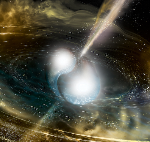
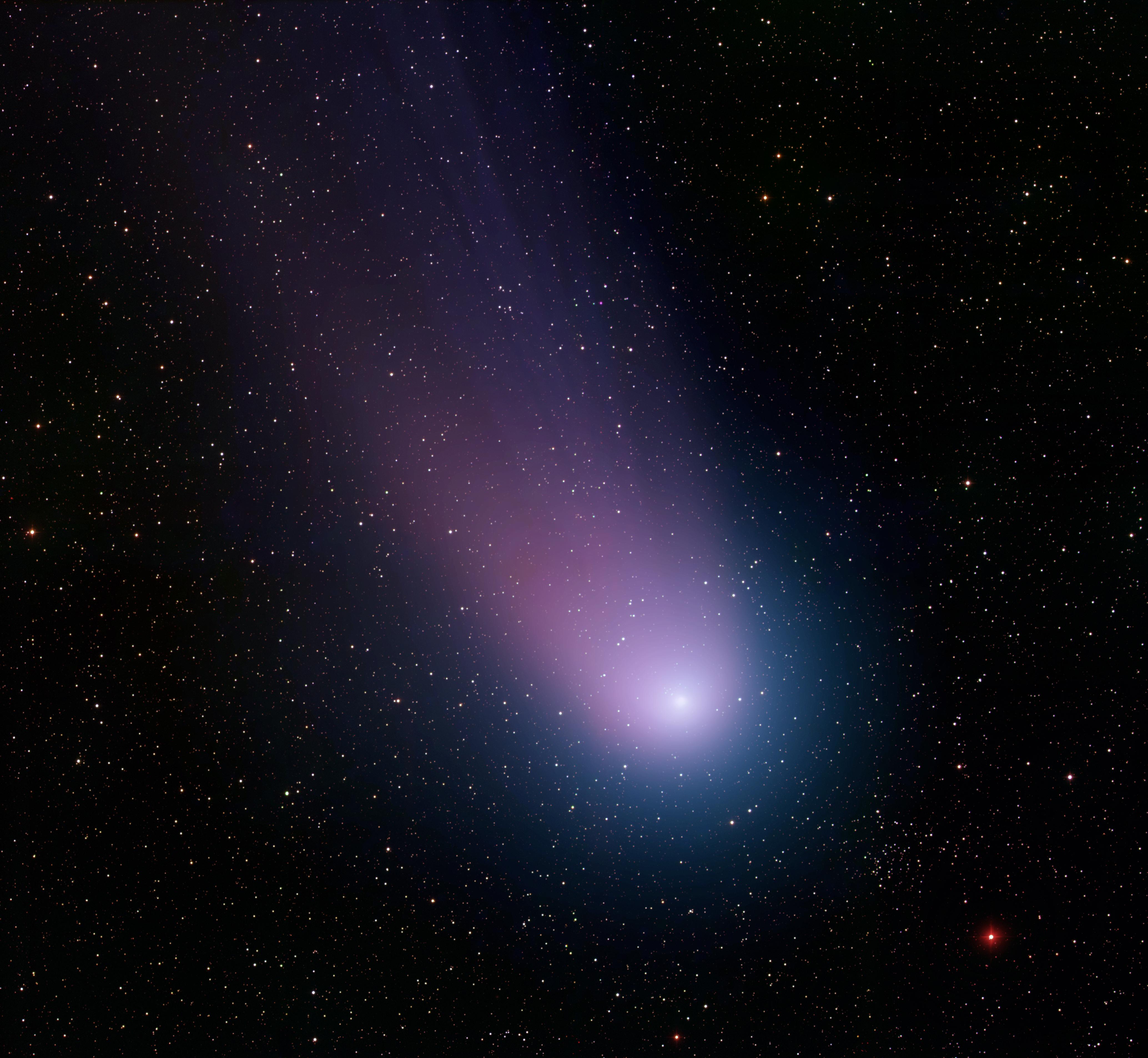
Artist’s impression of the electromagnetic signal from the merger of two neutron stars. [National Science Foundation/LIGO/Sonoma State University/A. Simonnet]
The event captured in August 2017, known as GW170817, is one of just two binary neutron star mergers we’ve observed with LIGO and its European sister observatory Virgo so far. But these collisions are likely to become a common detection in the future, particularly as LIGO and Virgo continue to upgrade and approach their design sensitivity.
Reducing the Lag
In the case of GW170817, interferometer glitches and data transfer issues prevented an alert from going out until 40 minutes after the merger. By the time follow-up telescopes had been advised where to search for the collision, the relevant region of the sky was below the horizon; the first manual follow-up couldn’t be conducted until nearly 8 hours after the merger.
To capture a neutron star merger without this delay, we’ll clearly need reduce the alert lag time — but could LIGO send out alerts even before the neutron stars collide? A study led by Surabhi Sachdev (The Pennsylvania State University) has recently demonstrated that a LIGO data analysis pipeline will be capable of providing advance warning for some future mergers.
Early Warning
Sachdev and collaborators analyze the performance of GstLAL, an early warning gravitational-wave detection pipeline for LIGO/Virgo that looks for signals of neutron star binaries approaching merger.
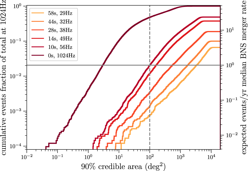
Cumulative distributions of the sky localizations of injected binary neutron star merger signals recovered by the authors’ pipeline. Results show that at least one event per year will be detected before merger and localized to within 100 deg2. [Sachdev et al. 2020]
A Well-Notified Future
Sachdev and collaborators predict that when LIGO and Virgo reach their design sensitivity, nearly 50% of total detectable mergers will be spotted at least 10 seconds before merger — a total that amounts to perhaps 6 to 60 events per year, depending on the neutron star merger rate.
With rapid localization and quick relay times for alerts, this early-warning system could provide follow-up telescopes with the opportunity to capture neutron-star mergers in real time, as they happen. Such observations would provide insight into what magnetic conditions are like around the neutron stars, how heavy elements are synthesized, and whether binary neutron stars are the source of fast radio bursts.
Citation
“An Early-warning System for Electromagnetic Follow-up of Gravitational-wave Events,” Surabhi Sachdev et al 2020 ApJL 905 L25. doi:10.3847/2041-8213/abc753


