Features Archives - Page 58 of 112

Features RSS

12 June 2020

Seeing Things in Threes

GW Ori is a system of three stars that are gravitationally bound. Aside from being a triple system, GW Ori also stands out for another reason — it harbors a circumtriple disk, which is a disk of gas and dust surrounding all three stars.

A Tricky Triple

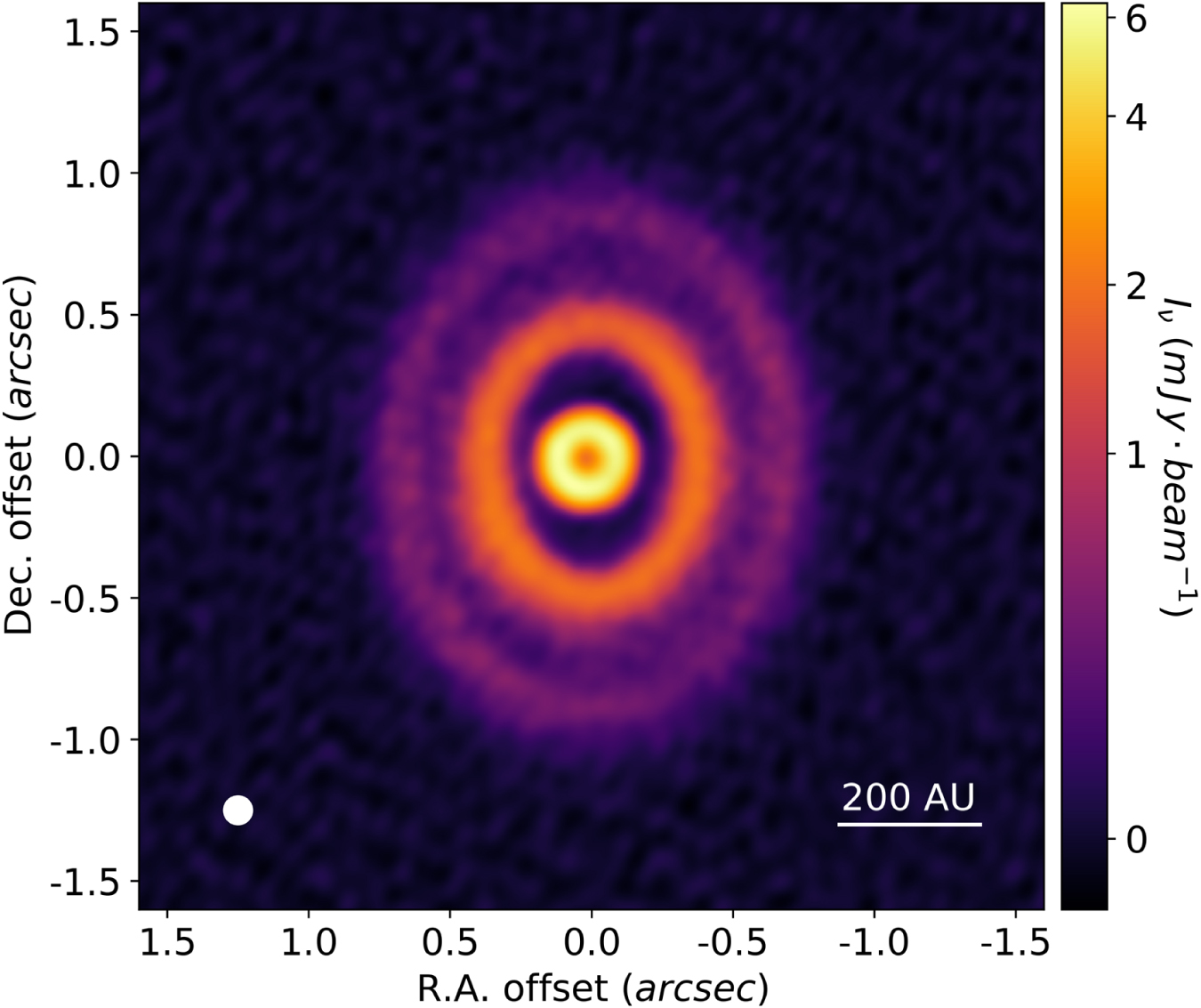
The dust component of GW Ori’s disk as seen by ALMA, showing the three rings discussed in this study. The x- and y-axes of the plot are position offsets, with (0,0) being the position of GW Ori. The color of the rings indicate intensity of emission, with yellow being more intense than purple. The circle in the lower left corner shows the size of the beam used by ALMA to image the disk. [Bi et al. 2020]

GW Ori lives in a star cluster called Lambda Orionis, which appears near Betelgeuse on the sky. The inner stars of the system, GW Ori A and GW Ori B, orbit each other and are separated by about 1 astronomical unit (au). The third star, GW Ori C, revolves around its two companions at a distance of roughly 8 au.

GW Ori’s circumtriple disk is enormous relative to the orbits of its stars. The dust component of the disk is about 400 au across, with the gas component spanning roughly 1,300 au. For scale, Neptune is only about 30 au from the Sun!

Models of GW Ori have suggested a gap in the disk between 25 and 55 au from its center. A recent study led by Jiaqing Bi (University of Victoria) attempted to test these models and probe the structure of GW Ori directly using observations by the Atacama Large Millimeter/submillimeter Array (ALMA).

Finding Rings in Radio

Bi and collaborators used ALMA observations taken at multiple frequencies to probe the gas and dust of the circumtriple disk. The dust component has characteristic emission that can be observed at 1.3 millimeters, while the gas can be studied using a particular transition of carbon monoxide.

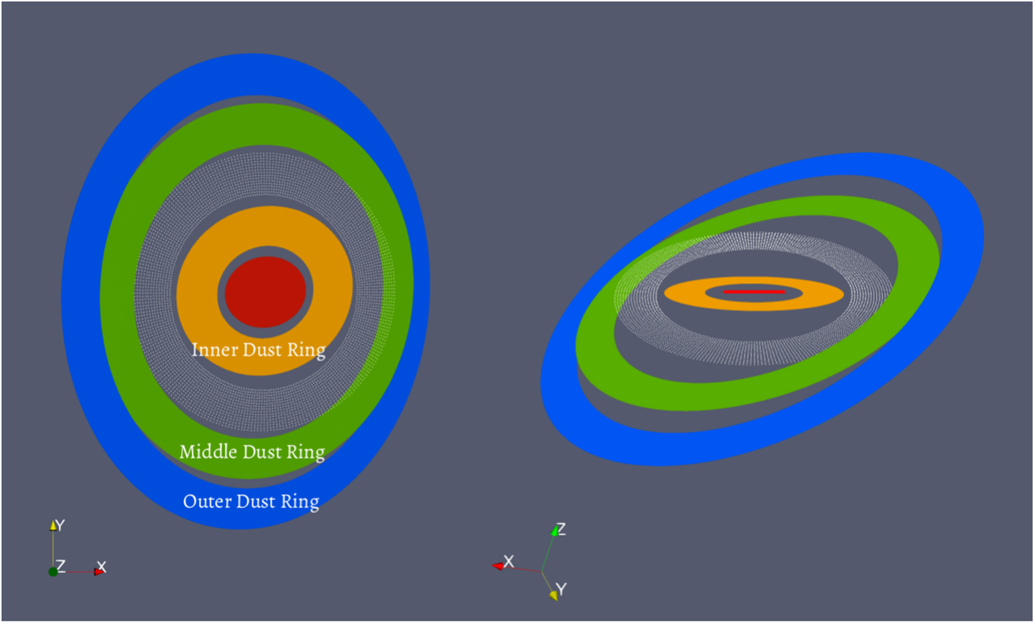
A schematic showing the likely alignment of GW Ori’s dust rings. The diagram on the left is how the disk appears on the sky and the diagram on the right is how the disk would appear if seen edge-on. The red ellipse is the plane of the orbits of GW Ori AB and GW Ori C. The ring of white dots represents the gap between the inner dust ring and middle dust ring. The orientation axes for both diagrams are located in their respective lower left corners. [Bi et al. 2020]

The gas observations showed the expected disk rotation, and additional structure in the disk was immediately apparent in the dust observations. Bi and collaborators identified three dust rings in GW Ori’s disk at roughly 46, 188, and 338 au from its center, the innermost ring being the one that was suggested by past models. Additionally, an unexpected result was brought to fore — the dust rings may be very misaligned relative to one another!

Out of Balance But It’s Fine

Bi and collaborators found that the dust rings showed significant inclinations relative to the plane of the orbit of GW Ori A and B — specifically 11, 35, and 40 degrees starting from the innermost ring. The gas observations back this up, requiring a model that assumes some distortion from an undisturbed disk.

Additional analysis and simulations by Bi and collaborators suggest that the stars of GW Ori alone could not be responsible for this misalignment. The innermost ring also adds another puzzle to this system: in addition to being misaligned, it also has a non-zero eccentricity, meaning its center is different than those of the other rings.

A possible explanation could be additional companions to GW Ori, which are also carving out paths in the disk. This phenomenon has been observed by ALMA before in protoplanetary disks. If this is the case, it would be the first time circumtriple companions were detected. Only time will tell!

Citation

“GW Ori: Interactions between a Triple-star System and Its Circumtriple Disk in Action,” Jiaqing Bi et al 2020 ApJL 895 L18. doi:10.3847/2041-8213/ab8eb4

27 May 2020

Are We Watching a Planet Disintegrate?

Among the wealth of exoplanets we’ve discovered beyond our solar system, some are temperate, some less so. New observations have now revealed what may be a particularly inhospitable environment: a planet literally disintegrating as it orbits its host.

Peering Through the Shroud

Artist’s illustration of another DMPP-discovered planetary system, DMPP-2. [Mark A. Garlick/Haswell/ Barnes/Staab/Open University]

With initial observations in 2015, the Dispersed Matter Planet Project (DMPP) promised an innovative approach to hunting for exoplanets closely orbiting their hosts. Using high-cadence, high-precision radial velocity measurements, the project targets bright nearby stars that shows signatures of being shrouded in hot circumstellar gas. By looking for tiny radial-velocity wiggles in the star’s signal, the DMPP team hopes to detect small planets that are losing mass as they orbit close to their hot hosts.

In December 2019, DMPP announced its first discoveries: six planets orbiting around three different target stars. Now, in a new publication led by scientist Mark Jones (The Open University, UK), the team has revisited the first of these systems, DMPP-1, with follow-up photometry from the Transiting Exoplanet Survey Satellite (TESS).

Intriguingly, the radial-velocity-detected planets are not the only signals from this system.

Missing the Expected, but Finding the Unexpected

DMPP-1 is a 2-billion-year-old star located just over 200 light-years away. The radial-velocity observations of this system revealed the gravitational tugs of four planets all orbiting with periods of less than 19 days. The radial-velocity data suggest that this system is probably near edge-on and contains three super-Earths and one Neptune-like planet.

Phase-folded TESS light curve for DMPP-1, identifying a weak transit signal with a period of P = 3.2854 days. [Jones et al. 2020]

Jones and collaborators began their photometric follow-up by searching TESS data for evidence of these four planets transiting across the host star’s face. Interestingly, they found no sign of transits at the predicted periods — indicating that the four radial-velocity planets are either smaller than expected, or that the system isn’t quite edge-on after all, so the planets don’t pass directly in front of the star.

The authors did, however, find a new signal: a weak transit detection with a period of just ~3.3 days. This signal doesn’t match any of the known radial-velocity planets.

A Disappearing Planet?

What might this marginal detection be? Its variable transit depths, short period, and apparent small size are all consistent with a catastrophically disintegrating exoplanet — a close-in, small, rocky planet that is so irradiated by its host that its rocky surface is being sublimated. As time goes on, such a planet will eventually disintegrate into nothing.

The depths of the seven detected transits are highly variable, with one even consistent with a depth of zero! This variability is common for disintegrating planets, as the cloud of ablated material is the primary cause of the transits. Click to enlarge. [Jones et al. 2020]

This transit signal still needs to be confirmed with additional follow-up photometric observations. Assuming it proves to be a true detection, however, such a disintegrating, rocky planet orbiting a bright nearby star would provide a veritable gold mine of information.

By exploring the transit signals from DMPP-1 with future technology like the James Webb Space Telescope, we will be able to examine the composition of the ablated material, potentially revealing clues as to how hot, rocky inner planets form and evolve.

Citation

“A Possible Transit of a Disintegrating Exoplanet in the Nearby Multiplanet System DMPP-1,” Mark H. Jones et al 2020 ApJL 895 L17. doi:10.3847/2041-8213/ab8f2b

22 May 2020

Making Galaxies of All Sorts

It’s hard to translate an image taken by a telescope to a physical object like a galaxy, but, like with most things, computers have made the job easier. Astronomers can code models of galaxies and determine the most realistic models based on observations. A recent study showcases this, presenting a code that can model all sorts of galaxies along with their internal motions.

Hubble view of NGC 1300, a barred spiral galaxy. [NASA, ESA, and The Hubble Heritage Team (STScI/AURA)]

Physical Frameworks and Altered Orbits

Any model begins with some assumed framework of physics. In a 1979 paper, Martin Schwarzschild proposed a method of modeling groups of stars called the orbit-superposition method. This method assumed that a system could be modeled as a gravitational potential that had objects orbiting in it and that properties of the system could be studied by seeing how the orbits changed with time.

While Schwarzschild used the orbit-superposition method to consider elliptical galaxies, other researchers have used it to study galaxies with more distinct structures like disks and bars. Since the 1990s, the Schwarzschild orbit-superposition method has been used extensively in galaxy modeling.

In a new study, Eugene Vasiliev (University of Cambridge) and Monica Valluri (University of Michigan) present a new code called Forstand, an implementation of the Schwarzschild method that can be applied to all sorts of galaxies without excessive computational cost.

An example of modeling results (top) and mock kinematic data (bottom). In the results plot, β and α describe the orientation of the mock galaxy. Ω is pattern speed and ɣ is mass-to-light ratio. The gray dots are the models considered and the red cross is the true value. The blue contours show the likeliest values for the pattern speed and mass-to-light ratio. The mock data plot is a velocity map, highlighting the x-, y-, and z-axes. The velocities changing from negative to positive indicates that the galaxy is rotating. [Adapted from Vasiliev & Valluri 2020]

Mockups of Mock Galaxies

The code was tested with two different data sets of mock galaxies — one that was low-resolution but spanned large regions of the component galaxies, and one that was high resolution but only covered the central regions of galaxies. The mock galaxies were all roughly the size of the Milky Way and had variations in their structure and orientation.

Vasiliev and Valluri assumed that the 3D shapes of their galaxies were known, acknowledging that this assumption can’t easily be made in the case of observational data. However, in all other ways the mock data were very similar to data taken by actual astronomical instruments.

The code was able to accurately recover the mass-to-light ratios and the pattern speeds of the mock galaxies. For galaxies, the mass-to-light ratio lets astronomers understand how much of the matter in a galaxy is dark matter. The pattern speed has to do with how the overall structure of a galaxy — spiral arms, for example — moves.

Vasiliev and Valluri wrapped up with avenues for improvement on their code. Forstand wasn’t able to recover the properties of certain galaxy components, specifically central black holes and dark matter haloes. There’s also still the issue of determining 3D galaxy shapes, which can be tricky to constrain observationally.

However, room for improvement doesn’t take away from the fact that the Schwarzschild method is a powerful tool when it comes to modeling galaxies. And Vasiliev and Valluri seem to have come up with a code that makes the Schwarzschild method far more accessible than before.

Citation

“A New Implementation of the Schwarzschild Method for Constructing Observationally Driven Dynamical Models of Galaxies of All Morphological Types,” Eugene Vasiliev and Monica Valluri 2020 ApJ 889 39. doi:10.3847/1538-4357/ab5fe0

20 May 2020

Cosmic Rays as the Source of Life’s Handedness

You might expect living cells to be composed of a random soup of materials — but look closely and you’ll find they’re built from molecules with distinct orientation preferences. How did life’s preferred “handedness” arise?

Living Single-Handedly

Billions of years ago, perhaps on the barely solidified crust of young Earth, life somehow arose from non-living matter. Today, we still haven’t solved the puzzle of how this transition from non-living to living occurred — but nature has left behind some helpful clues, including the intriguing geometry of life’s building blocks.

This generic amino acid exists in both a left-handed and a right-handed form: all the same things are attached in the same order, but the two forms are mirror images and cannot be superimposed. If both forms exist, why is life built from only left-handed amino acids? [Public Domain]

Many organic molecules come in two forms: left-handed and right-handed versions that are mirror images of each other. Just as you can’t put a left-handed glove onto your right hand, the mirror images of these chiral molecules are distinct and cannot be superimposed.

But while the pre-biological soup of material on early Earth contained both left-handed and right-handed forms of chiral molecules, living organisms are homochiral: they’re built almost exclusively from left-handed amino acids and right-handed sugars and nucleotides, which preferentially construct right-handed DNA and RNA.

A Cosmic Influence

What determined the handedness of Earth’s life? Was it a random initial disequilibrium — perhaps an overabundance of right-handed nucleotides trapped in a prebiotic nursery — that was then copied to all subsequent life? Or might the bias only have arisen later, driven by an outside source?

In a new study, scientists Noemie Globus (New York University and Flatiron Institute) and Roger Blandford (Stanford University and KIPAC) explore how cosmic rays may have shaped the evolution of early life forms.

In this schematic, the authors illustrate how the decay of a cosmic ray proton produces a shower of spin-polarized particles. When these particles reach the Earth’s surface, they affect right-handed and left-handed molecules differently, imparting a chirality bias. [Adapted from Globus & Blandford 2020]

Mutating for Survival

Cosmic rays are highly energetic, charged particles that careen in from space and slam into the Earth’s atmosphere, producing a cascade of secondary particles that can reach the planet’s surface.

Irradiation from cosmic-ray cascades is thought to drive gene mutation in DNA — an exploratory process that is critical for evolution. Many successive gene mutations in the earliest stages of life likely allowed proto-life forms to adapt to their environment, increasing their complexity and their chances of survival.

Intriguingly, the physical force that governs cosmic-ray cascades naturally introduces a preferential handedness in the secondary particles that reach the planet’s surface. Could this handedness somehow have introduced homochirality for life forms?

Pick a Hand

Globus and Blandford propose a model in which prebiotic chemistry produced both of the mirror versions of DNA and RNA. As these proto-lifeforms worked to self-replicate and evolve, cosmic rays rained down, introducing minor mutations.

Prebiotic chemistry may have produced both the left-handed and right-handed forms of RNA (which the authors cleverly label “evil” and “live” to underscore their mirror-image nature). [Adapted from Globus & Blandford 2020]

The handedness of the cosmic rays caused a slight difference in the mutation rate of the two different chiral forms, giving a tiny edge to the right-handed DNA. Over many generations of self-replication, this small chiral bias eventually resulted in early life dominated by a single handedness.

Can we test this model? We might find supporting evidence from laboratory experiments that simulate the influence of cosmic-ray irradiation on bacteria mutation rates. And, of course, we can hope that we’ll one day explore life’s building blocks in samples from asteroids and other planets, further pinpointing what led to life as we know it.

Citation

“The Chiral Puzzle of Life,” Noemie Globus and Roger D. Blandford 2020 ApJL 895 L11. doi:10.3847/2041-8213/ab8dc6

11 May 2020

Signs of Collisions to Come

We know that when two neutron stars — the dense, compact cores of evolved stars — collide, they produce signals that span the electromagnetic spectrum. But could these binaries also flare before they merge, as well?

A Broad Range of Signals

Artist’s impression of the collision and merger of two neutron stars. [NSF/LIGO/Sonoma State University/A. Simonnet]

The discovery and follow-up of the gravitational-wave event GW170817, a collision of two neutron stars, provided the first direct evidence of the many forms of light that are emitted in these mergers. Between the instant of collision and the months that followed, observatories around the world recorded everything from high-energy gamma rays to late-time radio emission.

But emission might not be restricted to during and after the merger! A new study conducted by two researchers from the Flatiron Institute, Elias R. Most (also of Goethe University Frankfurt, Germany) and Alexander Philippov, explores the possibility that neutron star binaries may also produce flares of emission in the time leading up to their final impact.

This plot of the out-of-plane magnetic field density indicates the twist in flux tubes connecting the two neutron stars seen at the center of the plot. Here, an electromagnetic flare is launched from the binary after a significant twist has built up due to relative rotation of the right star. [Most & Philippov 2020]

What About Magnetic Fields?

In particular, Most and Philippov focus on how the magnetospheres of the two neutron stars — the magnetized environment surrounding each body — interact shortly before the objects collide.

The authors conduct special-relativistic force-free simulations of orbiting pairs of neutron stars in which each star is threaded with the strong dipole magnetic field expected for these bodies. The simulations then track how the stars’ magnetic fields evolve, twist, and interact as the bodies orbit each other.

A Twisted Fate

Most and Philippov find that dramatic releases of magnetic energy are a common outcome if the neutron stars orbit close enough to one another that their magnetospheres interact.

The authors show that the brightness of the flare luminosity depends only on how far apart the neutron stars are in the simulation: the smaller the separation, the brighter the flare. This dependence demonstrates that the flaring events are driven primarily by the energy stored in the twisted tube of magnetic flux that forms connecting the two neutron stars.

Here, the twisted flux tube and resultant flaring is caused by orbital motion of 45° misaligned magnetic fields, rather than by one star spinning. The bottom panel shows a 3D visualization of the field line configuration at the time of flaring. [Most & Philippov 2020]

When the two neutron stars spin at different speeds, the magnetic field loop that forms between the stars becomes progressively more twisted — until this stored rotational energy is abruptly ejected. And even if neither neutron star is spinning, the authors show that magnetic flux twist still builds up and releases as a result of the binary’s orbital motion, assuming that the magnetic fields of the two stars are not aligned.

Look for Radio Clues

So can we observe these sudden releases of energy? Most and Philippov argue that we should be able to spot the drama in radio emission: a radio afterglow will be produced behind the magnetized bubble that’s ejected from the twisted loop, and additional radio emission can be produced when the bubble collides with surrounding plasma.

Future work on this topic will explore the impacts of the neutron stars’ inspiral, and how the interactions of the magnetospheres change when the neutron stars carry unequal charge. The current study, however, indicates it’s worth keeping a radio eye out to see if we can spot signs of collisions to come!

Citation

“Electromagnetic Precursors to Gravitational-wave Events: Numerical Simulations of Flaring in Pre-merger Binary Neutron Star Magnetospheres,” Elias R. Most and Alexander A. Philippov 2020 ApJL 893 L6. doi:10.3847/2041-8213/ab8196

8 May 2020

The Case of the Missing CO

Planets start their lives in disks of gas and matter around stars, so understanding these so-called protoplanetary disks is key to decoding planet formation. One interesting feature of protoplanetary disks is that they contain less carbon monoxide gas than the typical interstellar medium. When and how does this deficit arise?

Radio observations of the disk around the star DG Tau, with separate plots for each form or isotopologue of CO. The contours designate varying intensity and the colors indicate the velocity of the gas (red is faster than blue). The arrows in the bottom-most plot indicate outflows associated with DG Tau. [Adapted from Zhang et al. 2020]

Protostellar to Protoplanetary

Carbon monoxide (CO) is one of the most common compounds found in space and can be used to trace other chemical compounds along with the structure and mass distribution of objects. However, protoplanetary disks appear to lack CO gas to a startling degree relative to the interstellar medium (ISM). CO gas can be destroyed by chemical processes or be frozen out of the gas state, but these mechanisms alone can’t explain the deficit of CO gas seen in protoplanetary disks.

Protoplanetary disks are an evolved form of protostellar disks, which are created when a cloud of gas collapses to birth a star. Could CO be dissipated at this earlier protostellar disk stage? Or does the depletion only occur when the disk is older?

This question of timing is what motivated a recent study by a group of researchers led by Ke Zhang (University of Michigan). Zhang and collaborators used radio observations of three young (less than a million years old) protostellar disks to measure their levels of CO gas and compare them to that of the typical ISM.

COuld It Be at a Higher Level?

Zhang and collaborators selected their disks based on whether the disk structure could be seen in radio observations. They searched for three different forms of CO that, taken together with models, could probe the CO content of the entire disk. Different models were used to fit the disks, with adjustments to parameters like the gas-to-dust ratio and levels of molecular hydrogen.

The CO content and ages of various protostellar and protoplanetary disks. The average ISM value is shown for comparison. The disks used in this study are TMC1A, HL Tau, and DG Tau. The circles indicate disks and the squares indicate the average value for disks in star-forming regions. Disks younger than 1 million years are considered protostellar disks and disks older than one million years are considered protoplanetary disks. Click to enlarge. [Zhang et al. 2020]

Zhang and collaborators found that the CO gas content of all three protostellar disks is similar to that of the ISM. This puts them at a higher level relative to disks that are older than a million years.

What does this mean for the missing CO problem? The dropoff in CO appears to occur around the million year mark. This means that the CO depletion process is fairly rapid — on astronomical scales — and puts tight constraints on the responsible mechanisms.It also restricts the depletion to occurring within the disk rather than in the surrounding envelope of infalling gas.

It may take exploring combinations of physical and chemical processes to solve this puzzle, as well as observing a larger sample of disks. Either way, CO continues to be a useful molecule to find (or not find) in space!

Citation

“Rapid Evolution of Volatile CO from the Protostellar Disk Stage to the Protoplanetary Disk Stage,” Ke Zhang et al 2020 ApJL 891 L17. doi:10.3847/2041-8213/ab7823

6 May 2020

Build Your Own White Dwarf Photosphere

Have you ever wanted to examine the photosphere of a white dwarf up close and personal? Now you, too, can recreate and observe the atmospheric conditions of these extreme, dense, dead stars — assuming you have access to Sandia Labs’ Z Machine.

Extreme Cores

The eye-catching planetary nebula NGC 2440 surrounds a newly formed white dwarf star. [NASA/ESA and The Hubble Heritage Team (AURA/STScI)]

When a low-mass star exhausts its nuclear fuel, it ends its life by puffing off its outer layers. The dense, scalding hot core of the star — a white dwarf — is then left exposed, emitting high-energy radiation as it gradually cools.

White dwarfs are of enormous astronomical use to scientists. By observing white dwarfs, we are able to learn about topics ranging across stellar evolution, mass-loss processes, distances to astronomical objects, and even the age of the universe. To make correct inferences, however, we need accurate measurements of these white dwarfs’ masses — which is easier said than done.

Confusing the Scale

There are multiple techniques that can be used to measure the masses of white dwarfs. One of the most widely used and broadly applicable is spectroscopy: by fitting the absorption lines observed from white dwarfs’ hydrogen atmospheres with line shape models, we can estimate the surface gravity of the white dwarf, which can then be converted into a mass.

The catch? Masses measured this way don’t agree with masses measured using other techniques. So what’s going wrong?

Schematic illustrating the sample cell of hydrogen gas. Incoming X-rays heat the gold wall and backlighter, causing them to emit radiation and turning the hydrogen gas into a dense plasma similar to that of a white dwarf photosphere. Along the red line of sight shown, scientists can measure the absorption spectrum of the plasma. [Schaeuble et al. 2019]

It’s hard to answer this question without an independent and careful look at the spectral lines created by hydrogen absorption in white dwarf atmospheres. Conveniently, there’s a way of getting this detailed and controlled view: by recreating a piece of a white dwarf in a laboratory!

To Create a Star

The Sandia Z machine, located in Albuquerque, New Mexico, is the world’s most powerful radiation source. Using this machine, a team of researchers led by Marc-Andre Schaeuble (Sandia National Laboratories) pummeled a cell of hydrogen gas with high-energy X-rays to produce an extremely hot, dense plasma, simulating the conditions in the photosphere of a white dwarf.

Schaeuble and collaborators measured the absorption spectra that formed as radiation emitted from a backlighter was absorbed by this dense hydrogen plasma. The authors then extracted the atmospheric electron density — a measurement that relates to inferred stellar mass — by fitting hydrogen line shape models to these spectra.

A Discrepancy of Lines

Top: sample line profile fits to the Hβ and Hγ absorption lines using hydrogen line calculations. Bottom: electron density inferred from fits to the Hβ line (red) is consistently higher than that inferred from the Hγ line (blue). [Schaeuble et al. 2019]

Interestingly, this carefully controlled experiment showed the same issues with mass inference that we encounter using real white dwarf observations.

Schaeuble and collaborators show that they get a different outcome for the electron density depending on which absorption line the hydrogen line shape models are fit to: from the Hβ absorption line, they infer an electron density that’s >30% higher than that inferred from the Hγ absorption line. This discrepancy would translate into significantly different mass measurements for the same white dwarf.

So which fit — if any — is correct? We don’t know yet! These experiments indicate that current hydrogen line shape models don’t capture all the intricacies at play. By continuing to study white dwarfs — both of the natural and build-your-own varieties — we may yet puzzle it out.

Citation

“Hβ and Hγ Absorption-line Profile Inconsistencies in Laboratory Experiments Performed at White Dwarf Photosphere Conditions,” M.-A. Schaeuble et al 2019 ApJ 885 86. doi:10.3847/1538-4357/ab479d

1 May 2020

Challenging a Plasma Assumption

Simplifying a problem to make it solvable is a classic trademark of scientific modeling. But what happens when cows simply aren’t spheres?

The Perpetual Struggle: Accuracy vs. Feasibility

Theoretical models can fall into the trap of becoming spherical cows — they assume simplifications that render them no longer realistic. [Ingrid Kallick]

Theoretical models are critical in astronomy: telescope observations can only take us so far without the models that allow us to interpret them.

A major challenge for theorists is to develop models that are as realistic as possible, but are still simple enough to be solvable. This often requires making simplifying assumptions, turning complex systems into spherical cows. At times, these assumptions might be good approximations. At other times, they might be oversimplifications that cause us to misinterpret observations.

In a recent study, scientist Jack Scudder (University of Iowa) challenges an especially long-standing assumption used in many models of astrophysical and space plasmas.

Equilibrium or No?

Astrophysical and space plasmas are soups of ionized gas found throughout the universe, from supernova remnants to the intergalactic medium, from the Sun’s atmosphere to Earth’s magnetosphere. We can observe the photons emitted by these plasmas, and with the help of theoretical models, we can use these observations to remotely infer the properties of the astrophysical kitchens in which they were made.

Simulation showing a 2D gas relaxing toward a Maxwellian distribution as its particles collide. [Dswartz4]

But what these photons tell us depends on key simplifying assumptions in our models — and one of the most common assumptions is that of local thermodynamic equilibrium (LTE). The LTE approximation assumes that the photons we observe originated in a region where particles bounce around frequently, colliding with one another and taking on what’s known as a Maxwellian distribution of particle speeds in the process.

Is the LTE approximation reasonable to assume for astrophysical and space plasmas? Scudder argues that it often isn’t, especially in astrophysics where gravity requires strong spatial gradients in plasma properties that aren’t permitted in thermodynamic equilibrium. This means we’re likely interpreting observations incorrectly.

A New Solution

So if LTE isn’t a good approximation, what should we be using instead? Scudder has developed a model he calls SERM — Steady Electron Runaway Model — that generalizes the Maxwellian distribution for astrophysics, but reduces to it when spatial gradients are presumed absent. This model, he says, can be used to interpret observations of plasmas that are not necessarily in LTE.

To test his model, Scudder applies it to experimental measurements of the solar wind — the plasma streaming off of the Sun’s surface and suffusing interplanetary space. He shows that SERM predictions neatly match observations, and the model additionally explains a number of odd solar wind features that have puzzled scientists for decades.

A view of the solar corona during the 2015 total solar eclipse in Svalbard, Norway. [S. Habbal, M. Druckmüller and P. Aniol]

This model also shows promise, Scudder notes, for providing answers to other longstanding mysteries relating to astrophysical and space plasmas, such as the question of how the Sun’s outer atmosphere — its corona — is heated.

There’s more work to do to flesh out this model, and it is admittedly more complicated to work with than models that rely on the simplifying assumption of LTE. But Scudder’s work shows that SERM may be the next step needed in theoretical modeling to move the field forward.

Citation

“Steady Electron Runaway Model SERM: Astrophysical Alternative for the Maxwellian Assumption,” J. D. Scudder 2019 ApJ 885 138. doi:10.3847/1538-4357/ab4882

29 April 2020

Spins Point to How Black Hole Binaries Formed

Before stellar-mass black holes merge in a spectacular burst of gravitational waves, they’re locked in a fatal dance around each other as a binary black hole. A new study uses clues from black hole spins to explore how these binaries came to be paired together in the first place.

To Build a Binary

The Hanford (top) and Livingston (bottom) LIGO facilities, which work together to detect gravitational-wave signals. [Caltech/MIT/LIGO Lab]

With ten detections of merging stellar-mass black holes made by the LIGO/Virgo gravitational-wave observatories in just their first two observing runs, these detectors have opened a new window through which we can study the evolution of massive stars.

Among the open questions we hope to answer with these and future detections is the following: How were these binary pairs of stellar-mass black holes created? There are two main formation channels proposed:

Field binary evolution
In isolation in the galactic field, the two members of a binary star system independently evolve into black holes, and they remain bound to each other through this process.
Dynamical assembly
Black holes are formed independently and then sink to the centers of high stellar density environments like globular clusters. There, dynamical interactions cause them to pair up and later get ejected from clusters as bound binaries.

Recent research suggests a combination of these two channels is likely at work to produce the black hole binaries we’ve observed. But what fraction of the LIGO/Virgo binaries are created by each channel?

A new study by scientist Mohammadtaher Safarzadeh (Center for Astrophysics | Harvard & Smithsonian; UC Santa Cruz) explores this so-called branching ratio.

Illustration of a pair of black holes with misaligned spins. [LIGO/Caltech/MIT/Sonoma State (A. Simonnet)]

Spinning an Origin Story

Safarzadeh relies on one primary clue: black hole spin. Due to conservation of angular momentum, black holes binaries that form via isolated evolution are likely to have positive black hole spins — the spins of the black holes will be in the same direction as the orbital rotation of the binary. In contrast, the chaos of dynamical assembly should result in binaries with randomly distributed spins.

Safarzadeh statistically models two populations of black hole binaries produced by these two formation channels and compares this model to LIGO/Virgo’s 10 observations of mergers from their first two observing runs. He’s careful to also take into account LIGO/Virgo’s observational biases — the detectors have an easier time observing binaries with positive effective spin.

Dynamics Weigh In

The author’s calculated posterior distribution on the parameter Q, the ratio of field binaries to the total number of observed black hole binaries, shows that contribution from the dynamical channel is more than 55% with 90% confidence. [Safarzadeh]

The result? Safarzadeh estimates that the contribution of the dynamical assembly channel to the total population of binary black holes is more than 55%, with 90% confidence — which means that random pairings of black holes in the chaotic centers of dense star clusters likely dominate the population of black hole binaries we’ve observed.

This outcome can be further refined as we increase our observed sample size — LIGO/Virgo’s third observing run, now being analyzed, is expected to contain perhaps dozens of additional systems, and future detections will hopefully add many more binaries to the list!

Citation

“The Branching Ratio of LIGO Binary Black Holes,” Mohammadtaher Safarzadeh 2020 ApJL 892 L8. doi:10.3847/2041-8213/ab7cdc

27 April 2020

Searching Pulsars for Planets

Are there more hidden exoplanets lurking around extreme pulsar hosts? A recent study explores a well-observed set of pulsars in the hunt for planetary companions.

Ushering in the Age of Exoplanets

An artist’s illustration showing a network of pulsars whose precisely timed flashes of light are observed from Earth. Could some of these pulsars host planets? [David Champion/NASA/JPL]

The first planets ever confirmed beyond our solar system were discovered in 1992 around the pulsar PSR B1257+12. By studying the pulses from this spinning, magnetized neutron star, scientists confirmed the presence of two small orbiting companions. Two years later, a third planet was found in the same system — and it seemed that pulsars showed great promise as hosts for exoplanets.

But then the discoveries slowed. Other detection methods, such as radial velocity and transits, dominated the emerging exoplanet scene. Of the more than 4,000 confirmed exoplanets we’ve discovered overall, a grand total of only six have been found orbiting pulsars.

Is this dearth because pulsar planets are extremely rare? Or have we just not performed enough systematic searches for pulsar planets? A new study led by Erica Behrens (The Ohio State University) addresses this question by using a unique dataset to explore rapidly spinning millisecond pulsars, looking for signs of hidden planets.

The Advantage of Precise Clocks

How are pulsar planets found? Pulsars have beams of hot radiation that flash across our line of sight each time they spin. The regularity of these flashes is remarkably stable, and when we observe them over long periods of time, we can predict the arrival time of the pulses with a precision of microseconds!

Sample periodograms for two pulsars. The top panel includes a simulated planet signal injected into the data, producing a strong peak at the planet’s orbital period. The bottom panel is an actual periodogram for one of the pulsars in this study, showing no evidence of a planetary companion. [Adapted from Behrens et al. 2020]

Because these pulses are so predictable, any perturbation that might change their timing can be measured and modeled. In particular, the presence of a companion body around the pulsar will cause both objects to orbit the system’s center of mass, introducing a periodic signature in the pulsar’s pulse arrival times. This fluctuation in the pulse timing allows us to measure the period and mass of potential companions.

A Multi-Use Dataset

To search for these signatures in pulse data, Behrens and collaborators turn to observations of 45 separate millisecond pulsars, which were made as part of the North American Nanohertz Observatory for Gravitational Waves (NANOGrav) project.

NANOGrav’s primary goal is to use the precise timing of these pulsars to measure the warping of spacetime caused by gravitational waves. But in the process of this work, the project has been carefully monitoring pulse arrival times for these pulsars for 11 years, producing a remarkably detailed dataset in which we can search for evidence of planets orbiting any of the 45 pulsars.

Pushing Down to Moon Masses

Lower limits of detectable masses in the 11-year NANOGrav data set, as shown with black lines. The colored data shows the masses of the least massive 10% of confirmed exoplanets we’ve detected with other methods. Pulsar timing provides the ability to detect remarkably low-mass companion bodies. Click to enlarge. [Behrens et al. 2020]

Looking for periodic signals in the data, Behrens and collaborators rule out the presence of planets that have periods between 7 and 2,000 days. By injecting simulated signals into the data, the authors show that their analysis is sensitive to companions with masses of less than the Earth — in fact, for some pulsars, they’ve eliminated the possibility of all companions with more than a fraction of the mass of our Moon!

This study shows the incredible power and sensitivity of extended pulsar monitoring in the hunt for small exoplanets. While it may well be true that pulsar planets are very rare objects, those out there can’t stay hidden for long.

Citation

“The NANOGrav 11 yr Data Set: Constraints on Planetary Masses Around 45 Millisecond Pulsars,” E. A. Behrens et al 2020 ApJL 893 L8. doi:10.3847/2041-8213/ab8121

Previous 1 … 56 57 58 59 60 … 112 Next