
Studying Near-Earth Asteroids with Radar
Some observatories — like the recently collapsed Arecibo Telescope in Puerto Rico — examine nearby objects by bouncing radio light off of them. A new study has now improved how we analyze these observations to learn about near-Earth asteroids.
Clues from Reflections
There’s plenty we can learn about the universe from passive radio astronomy, in which we observe the radio signals emitted by distant sources. But when it comes to objects that lie near the Earth, we have another option: active radio astronomy.
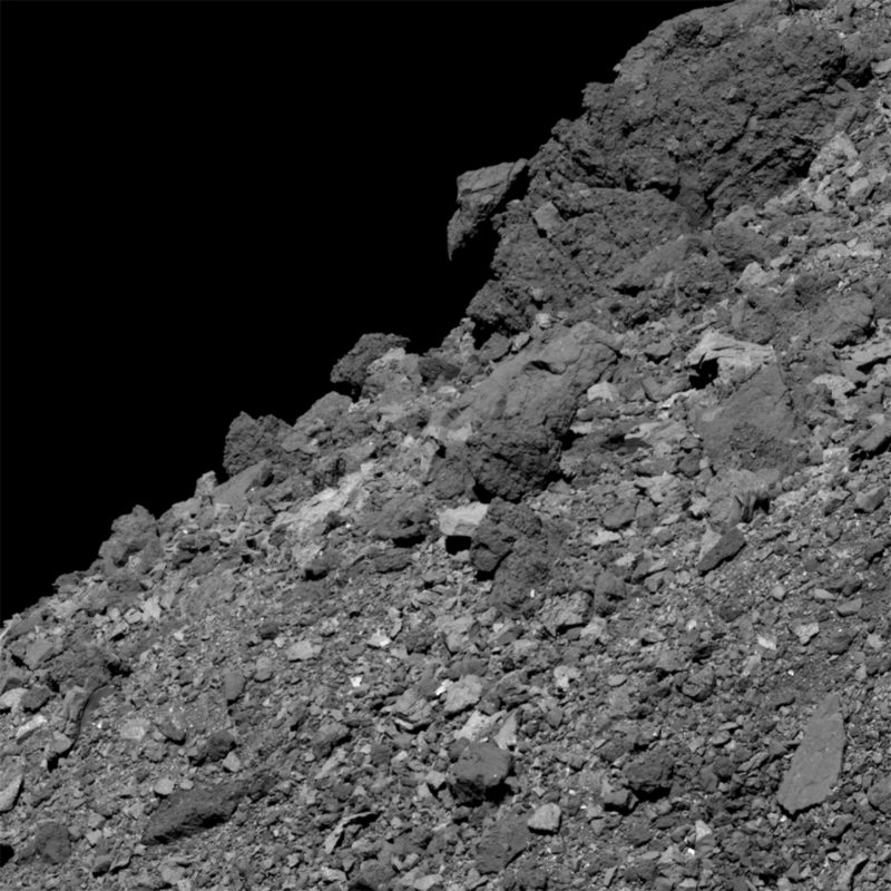
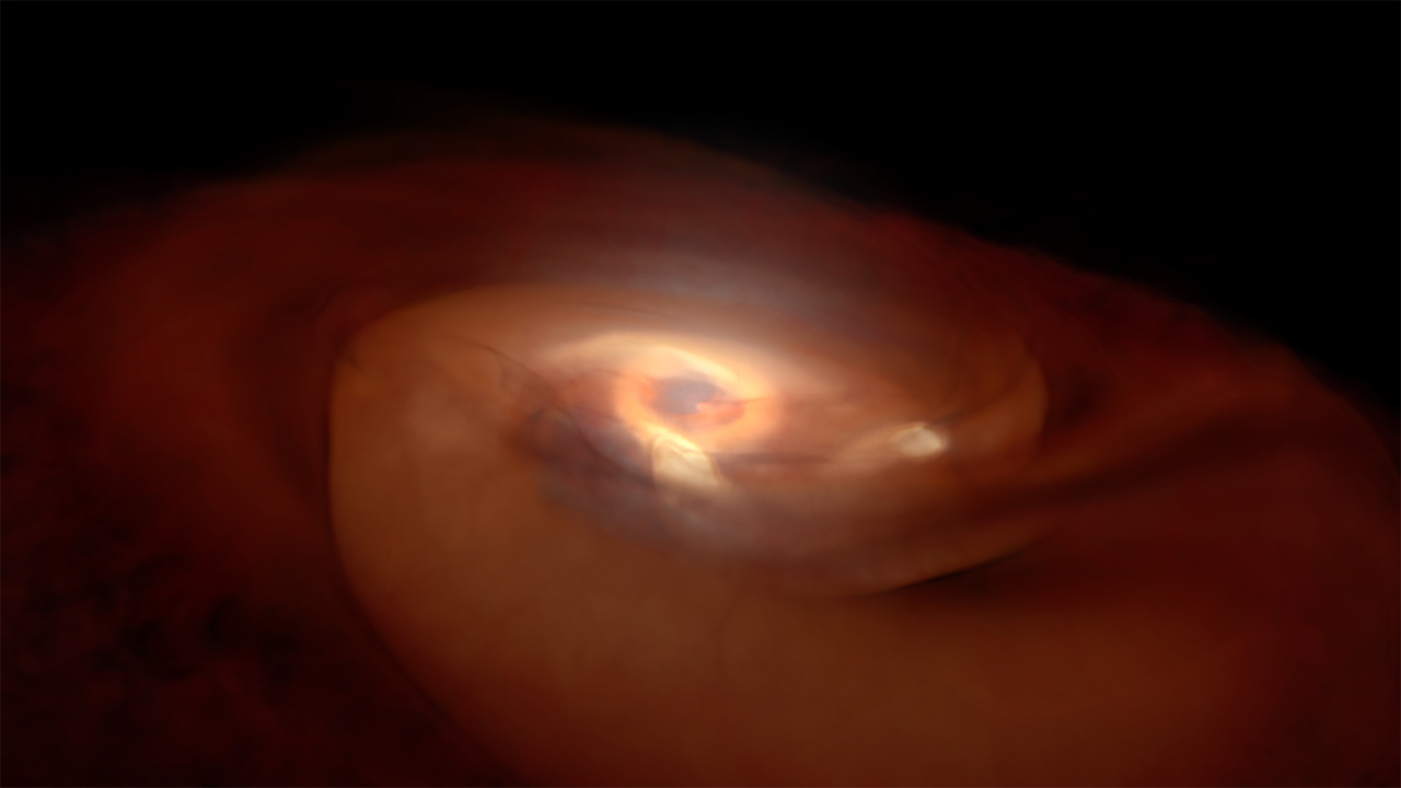
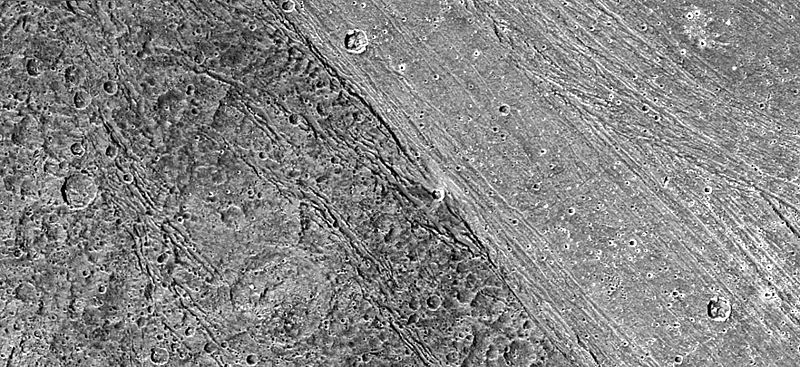
Asteroid surfaces are complex, as evidenced by this up-close image from OSIRIS-REx of the surface regolith of asteroid Bennu. [NASA]
What’s more, measurements of the polarization of the reflected light — the direction the light waves are vibrating — tell us about how the light was scattered from the surface and near-surface of the body. This, in turn, provides information about the outer material properties of the object. Does this material consist of fine-grained dust, or large boulders? How porous is it? How reflective?
The answers to these questions help us to comprehend the nature of bodies close to the Earth. This is especially useful in the context of near-Earth asteroids, where understanding the structure and composition of these potential hazards could be critical for mitigation tactics or spacecraft visitation.
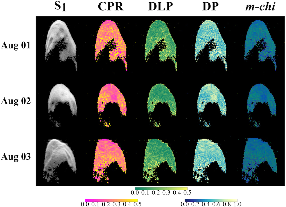
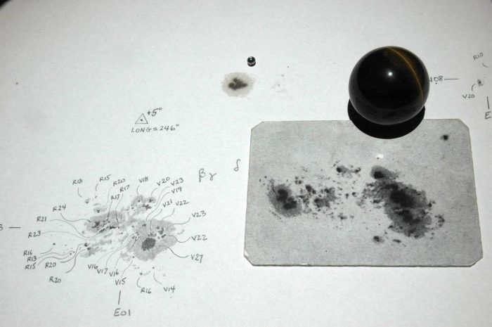
Radar data for near-Earth asteroid 1999 JM8, broken down into different polarization components for three different observation dates. [Hickson et al. 2021]
Separating the Pieces
The catch? Interpreting radar polarimetry isn’t easy. To disentangle the combined information about a body’s surface roughness, particle shape, ice content, boulder abundance, composition, and viewing geometry, we often make inferences based on well-characterized surfaces like the Moon’s. But when the surfaces we’re studying are more complex — like those of near-Earth asteroids — the lunar analog may not apply.
To address this, a team of scientists led by Dylan Hickson (Arecibo Observatory) recently developed an improved methodology to analyze the ground-based radar polarimetry of near-Earth asteroids. Hickson and collaborators show how we can decompose the reflected radio images of asteroids to derive specific polarimetric products, and they then use numerical simulations to improve their interpretations of these signals.
The authors apply their methodology to archived radar observations of three near-Earth asteroids obtained by Arecibo, demonstrating that they can retrieve a wealth of information about the physical properties of the asteroids’ surfaces using this approach.
An Uncertain Future

This plot shows the number of near-Earth asteroids detected by radar each year between 1980 and 2021 (last updated 4 February 2021). Despite the collapse of Arecibo (blue), we can still expect future detections from Goldstone (red). [NASA JPL]
Fortunately, we have archives that contain past data for more than 1,100 radar-detected asteroids and comets. Reanalysis of this content using the authors’ new methodology is certain to provide valuable information while the field of radar astronomy reshapes itself going forward.
Citation
“Polarimetric Decomposition of Near-Earth Asteroids Using Arecibo Radar Observations,” Dylan C. Hickson et al 2021 Planet. Sci. J. 2 30. doi:10.3847/PSJ/abd846


