
A Relic Black Hole in a Dwarf Galaxy
Using a new technique, scientists have identified a supermassive black hole lurking in a low-mass, low-metallicity galaxy. Could this discovery be just the tip of the iceberg?
Hunting for Seeds
How did the first supermassive black holes — black holes of millions or billions of solar masses — form?

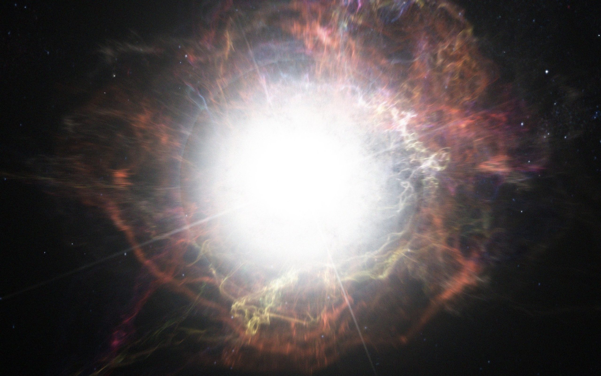
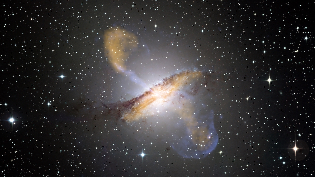
Artist’s illustration of a primordial galaxy dominated by the supermassive black hole in its center. [NASA/ESA/ESO/Wolfram Freudling et al. (STECF)]
To identify the seeds of supermassive black holes and address these questions, we need to explore the least-disturbed supermassive black holes that we can find today. Small, low-metallicity galaxies — those that have had a peaceful cosmic history, devoid of the mergers that drive significant black-hole growth — are thus the perfect targets to search for the relics of supermassive black hole seeds.
The catch? These are precisely the environments in which it’s difficult to spot black holes!
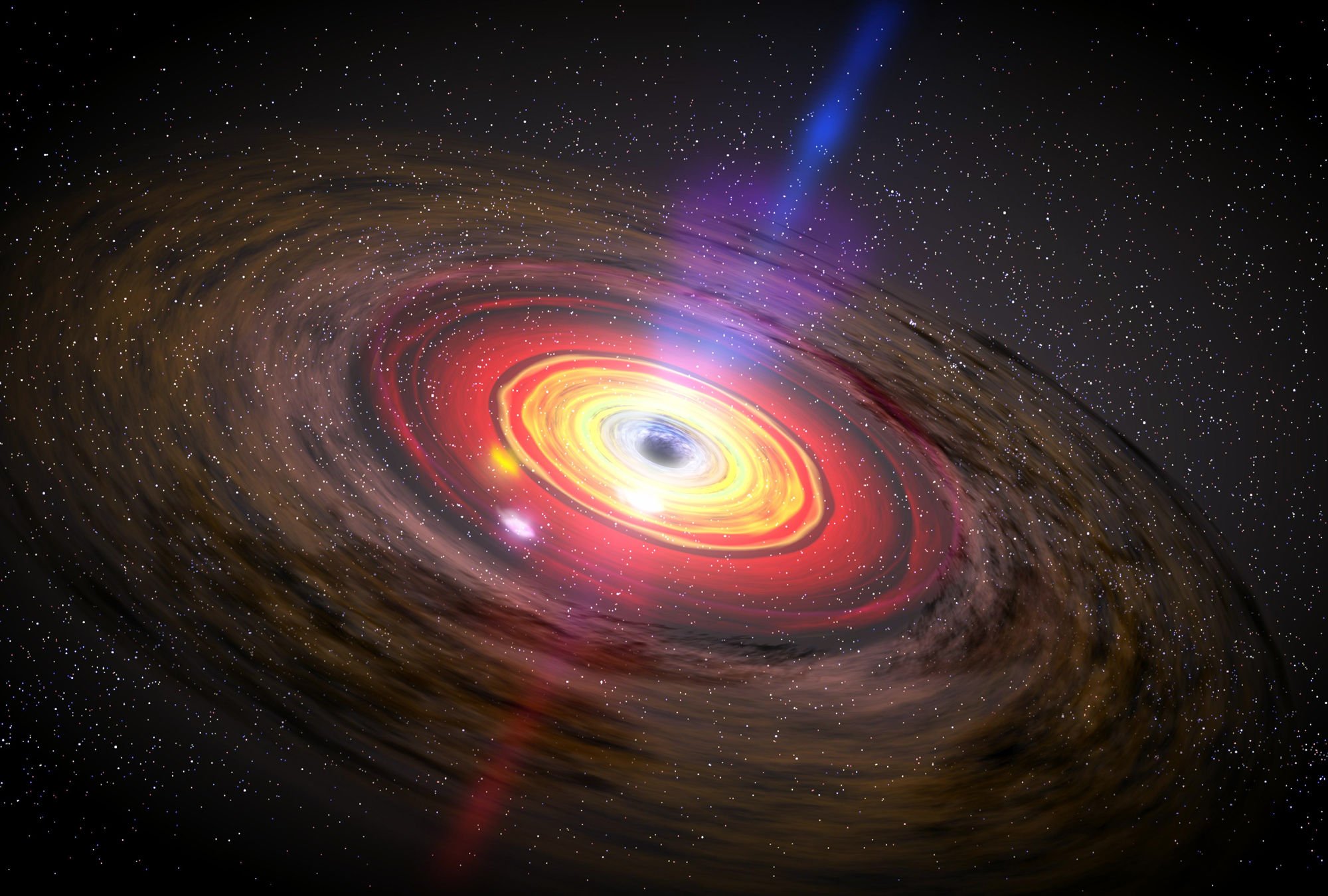
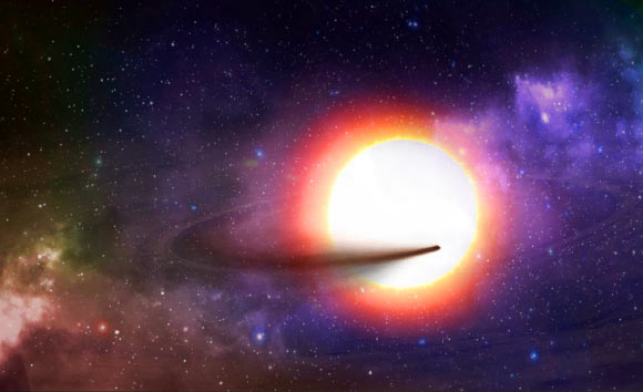
Artist’s depiction of the active nucleus of a galaxy, including an accretion disk spiraling around the supermassive black hole and jets of material flung out from both poles. [NASA/Dana Berry/SkyWorks Digital]
A New Approach
The easiest black holes to detect are those that are actively feeding, known as active galactic nuclei (AGNs). But the typical method for identifying an AGN — which relies on specific signatures in the source’s optical spectrum — is biased against low-metallicity and relatively merger-free galaxies, missing the precise population we want to find! Only a handful of AGNs have been identified in dwarf galaxies, and most of these lie in high-metallicity environments. So how do we find our seed relics?
According to a team of scientists led by Jenna Cann (George Mason University), it’s time for a different approach. Instead of relying on optical signatures, Cann and collaborators focus on finding coronal lines — near-infrared emission lines produced by ions that are excited by high-energy radiation. The presence of these lines can reveal a hidden AGN, even when a galaxy shows no sign of an AGN in optical emission.
Discovery of a Relic
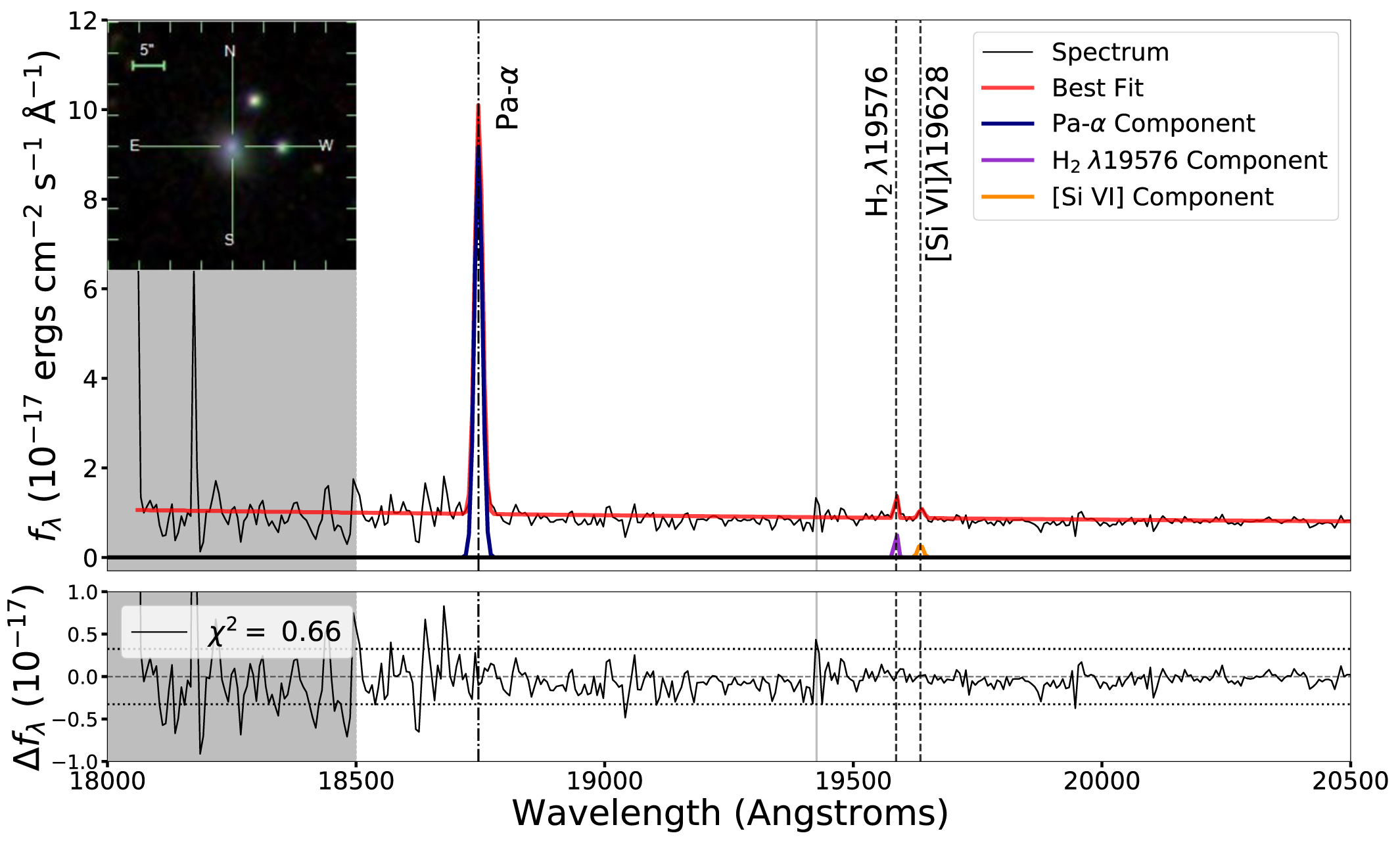
The near-infrared spectrum of J1601+3113, captured using the GNIRS instrument at Gemini North, shows the presence of the [Si VI] coronal line, the tiny orange bump on the right of the spectrum. This provides evidence of an AGN. [Adapted from Cann et al. 2021]
Cann and collaborators’ discovery marks the first time that an AGN has been identified in a low-mass, low-metallicity galaxy with no optical signs of AGN activity, underscoring how the coronal-line technique can help us find AGNs that might otherwise go undetected.
And with the James Webb Space Telescope scheduled to launch this year, we’ll (hopefully!) soon be collecting infrared spectra with unprecedented sensitivity. With any luck, we’re about to have access to a remarkable new population of lightweight AGNs hiding in small, low-metallicity galaxies — and with it, valuable insight into how these objects were born.
Citation
“Relics of Supermassive Black Hole Seeds: The Discovery of an Accreting Black Hole in an Optically Normal, Low Metallicity Dwarf Galaxy,” Jenna M. Cann et al 2021 ApJL 912 L2. doi:10.3847/2041-8213/abf56d


