Investigating a Bright Flare in a Nearby Galaxy
Astronomers have seen an extraordinarily bright, long-lasting radio flare in the center of a nearby galaxy. After investigating further they found evidence of a relativistic jet most likely caused by the immense gravitational pull of the galaxy’s supermassive black hole tearing a star apart.
An Unusual Signal

The radio flare VT J0243 was discovered using the Karl G. Jansky Very Large Array, located in Socorro, NM. [NRAO/AUI/NSF; CC BY 3.0]
Intrigued, Somalwar and colleagues conducted a series of follow-up observations across multiple parts of the electromagnetic spectrum. Radio observations revealed the presence of a powerful relativistic jet. The spectrum of the jet revealed it to be young. Whatever caused it must have happened fairly recently.
X-ray analysis hinted at the presence of an accretion disk of material in the galactic center. Matter falling from this disk into the black hole could account for the radio flares, and material corralled by the black hole’s magnetic field could launch the jet.

Active galactic nuclei can light up the radio sky — but VT J0243 doesn’t quite fit with a typical active galaxy picture. [NASA/JPL-Caltech]
Exploring the Options
The team examined two main possibilities for what happened. The first suggests a long-standing accretion disk that existed long before the flare was fired — in other words, this galaxy is an active galactic nucleus. However, if this picture is correct, the team says it isn’t clear what caused the accretion rate to suddenly spike and generate the flare. The energy distribution across the radio spectrum also differs from most other active galactic nuclei with young jets. If it is an active galactic nucleus, it would be an unusual one.

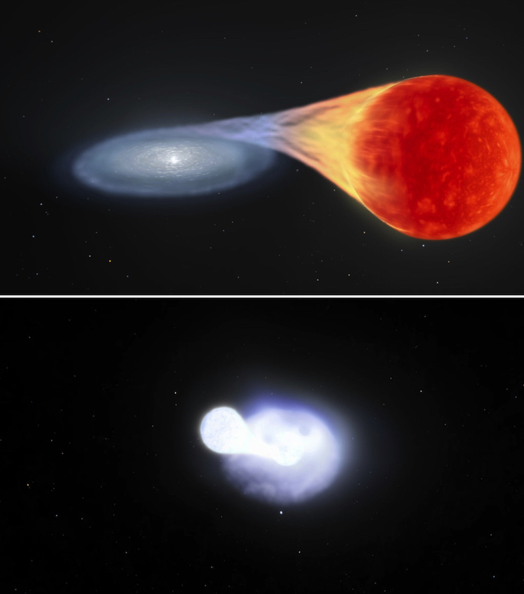
Artist’s impression of a tidal disruption event — the ripping apart of a star by a black hole. [NASA/JPL-Caltech]
For now it remains a mystery, but this discovery is a clarion call for astronomers ahead of an influx of data from the Very Large Array Sky Survey (VLASS). Started in 2017 and due to finish in 2024, this survey is trawling 80% of the sky and is expected to catalog approximately 10 million radio sources. Among them should be many young jets like the one associated with VT J0243. Perhaps then astronomers will better understand the true triggers of such dramatic radio flares.
Citation
“A Candidate Relativistic Tidal Disruption Event at 340 Mpc,” Jean J. Somalwar et al 2023 ApJ 945 142. doi:10.3847/1538-4357/acbafc


 Neutron Stars with a Dash of Dark Matter")