Features RSS

Illustration of an accretion disk swirling around a supermassive black hole

Astronomers have discovered a handful of supermassive black holes that are associated with bursts of X-rays that recur every few hours or days. New work expands on a theory that explains these X-ray outbursts and explores how we can spot them at other wavelengths.

Investigating Quasi-periodic Eruptions

For the past few decades, researchers have seen X-ray flares coming from the centers of certain galaxies. These flares, dubbed quasi-periodic eruptions, last about an hour, and individual flares are separated by a few hours to a few days. The brightness changes from flare to flare, and the flares don’t recur at precise intervals, giving the events their name. The cause of quasi-periodic eruptions isn’t yet known, but leading models involve a star being partially torn apart by a supermassive black hole or an object interacting with gas accreting onto a black hole.

diagram showing the star–disk–black hole model proposed by the authors

A simple diagram showing the proposed model. A star orbits a supermassive black hole on an orbit that is slightly elliptical (exaggerated here for clarity) and inclined relative to the accretion disk (yellow). The X’s mark the places where the star passes through the disk. The time between crossings at A and B is shorter than the time between crossings at B and A. [AAS Nova/Kerry Hensley]

Previously, Itai Linial (Institute for Advanced Study and Columbia University) and Brian Metzger (Columbia University and Flatiron Insitute) proposed a model that explained a curious feature seen in two quasi-periodic eruption sources: a repeating pattern in which pairs of flares are separated by alternating long and short intervals. In this model, a star near a supermassive black hole collides repeatedly with an accretion disk. The disk might form when the star loses gas to the black hole’s gravitational pull, or it might come from an unrelated star that’s being ripped apart. Each time the star plunges through the disk, shocks heat a spray of gas that emits an X-ray flare. If the star’s orbit is elliptical and inclined relative to the accretion disk, this model naturally explains why the flares aren’t precisely periodic: flares are more closely spaced when the star travels a shorter distance between disk crossings, and they’re farther apart when the star travels farther between crossings.

An Ultraviolet Possibility

Now, Linial and Metzger have explored the implications of this model further, delving into the properties of quasi-periodic eruptions to understand if these events can only be observed at X-ray wavelengths, or if it’s possible to see them at other wavelengths as well. Because there are several planned and proposed ultraviolet survey missions, the team focused on the possibility of observing quasi-periodic eruptions in the ultraviolet. By outlining the equations that describe a star punching through a thin disk of gas around a supermassive black hole, the authors predicted how the brightness and timing of the flares depend on the size and mass of the star, how quickly the black hole is accreting gas from the disk, and other factors.

plot summarizing the conditions under which quasi-periodic eruptions emerge in the X-ray versus the ultraviolet

Luminosity of quasi-periodic eruptions as a function of accretion rate. This plot demonstrates how a system might transition from producing X-ray flares to ultraviolet flares, or vice versa, as the accretion rate changes. Click to enlarge. [Linial & Metzger 2024]

To be able to spot a flare, it must outshine the hot, glowing gas of the disk, which may be possible in two cases. In the first, stars on short orbits around relatively massive black holes — in the few-million-solar-mass range — produce bright X-ray flares. In the second, stars on long orbits around less-massive black holes — in the few-hundred-thousand-solar-mass range — produce bright ultraviolet flares. It may even be possible for X-ray flares to reinvent themselves as ultraviolet flares after fading from view at X-ray wavelengths, or vice versa, as the system evolves: if the accretion disk formed out of a disrupted star, the accretion rate will eventually drop, shifting the peak of the flare emission from X-rays to ultraviolet over time. It’ll be fascinating to see these predictions tested when future ultraviolet surveys get underway!

Citation

“Ultraviolet Quasiperiodic Eruptions from Star–Disk Collisions in Galactic Nuclei,” Itai Linial and Brian D. Metzger 2024 ApJL 963 L1. doi:10.3847/2041-8213/ad2464

illustration of a white dwarf star accreting material from a companion

Accurate models of supernova spectra are typically pretty slow, but neural networks are both fast and capable of mimicking many other codes. Recently, a team used the latter facts to overcome the former challenge and created a set of neural networks capable of rapidly modeling real supernova data.

Complex Explosions

As one might expect when dealing with one of the most violent, rapid, and energetic processes in the universe, one must take great care when modeling a supernova. In the seconds, hours, and days after the initial explosion, many different processes unfold on many different scales: unstable elements birthed from the raw power of the eruption decay into more durable forms; heavy elements are accelerated to mind-boggling speeds; nearby material begins to glow as the temperatures approach values beyond comprehension. Each of these processes and others affect the spectra that we measure here on Earth, and each of them must be closely tracked in order to correctly explain our observations.

The immense complexity of the problem places large demands on the codes that simulate the aftermath of a supernova. Despite many different simplifications and approximations, the inescapable fact remains that each of these simulations take a lot of time to run. For example, one code named TARDIS requires about one CPU hour to transform inputs such as total luminosity, time after explosion, and the structure of the ejecta into an output model spectrum. For astronomers who want to compare their real data to potentially millions of models to find the best-fitting values for those input parameters, that runtime won’t cut it.

A recently adopted unspoken code among the astronomy community states that if one scientist says “complex model” and “slow runtime” three times fast, another will appear with a machine learning solution to the problem. A team led by Xingzhuo Chen, Texas A&M University, just published a neural-network-accelerated supernova inference framework that answers this latest call.

Neural Networks and Nickel

A loss vs. epoch plot, showing exponentially decreasing trends for several curves.

The training progress of the neural networks as a function of iterations through the training data. [Chen et al. 2024]

Chen and collaborators set out to model real Type Ia supernovae using neural networks capable of rapidly converting spectra into underlying physical parameters. The first step required creating and training the networks. To do this, the team fed TARDIS 108,389 different input values and compiled the resulting spectra into a training library. They then let several neural networks loose in this library and tasked them with learning how to convert the spectra into their original inputs, or essentially how to undo all of TARDIS’s hard work. After a few tens of iterations through the library, the networks could faithfully mimic TARDIS in reverse, and the team was left with a several networks capable of constraining different physical parameters when shown a spectrum.

The inferred nickel abundance over time for several real supernovae. The expected decay rate is shown in the solid line. [Chen et al. 2024]

The researchers then handed over about 1,000 spectra of about 100 distinct supernovae to their trained networks and analyzed the resulting predictions. One quantity they focused on was the nickel content of the ejecta and how it evolved over time. They found that for some supernovae, the radioactive nickel depleted at exactly the predicted half-life of the unstable isotopes. Others, however, either had nickel stick around for longer than expected or fade away faster than the familiar rate. Exactly why this might be is unclear, and the mismatched cases could point to issues with the approximations made by TARDIS itself, or with assumed spherical symmetry/smoothness of their ejecta model.

Even still, the authors state that their work “represent[s] a significant improvement in the quality of the spectral modeling of [supernovae] compared to similar models in the literature.” By using this technique of harnessing neural networks to speed up complex physical models, astronomers can look forward to many more breakthroughs that wouldn’t be possible without an AI-assisted boost.

Citation

“Artificial Intelligence Assisted Inversion (AIAI): Quantifying the Spectral Features of 56Ni of Type Ia Supernovae,” Xingzhuo Chen et al. 2024 ApJ 962 125. doi:10.3847/1538-4357/ad0a33

illustration of a planet orbiting an M dwarf and losing its atmosphere

Which planets are most likely to lose their atmospheres? New research finds a surprising relationship between planet size and atmospheric escape and suggests that the smallest planets aren’t losing their atmospheres the fastest.

The Role of Atmospheric Loss

illustration of Mars losing ions from its atmosphere during a solar storm

An illustration of Mars losing ions from its atmosphere during a solar storm. [NASA/GSFC]

Don’t panic, but Earth is slowly losing its atmosphere — very slowly, at a rate so small that the Sun will balloon into a red giant and engulf our planet long before its atmosphere is whisked away. Atmospheric escape is an unavoidable reality for any planet encased in gas, but around our calm, middle-aged star, atmospheric loss is minimal.

Other planets in distant star systems are not as lucky: pummeled by fierce radiation and howling stellar winds, many exoplanets will lose most or all of their atmospheres. A planet’s ability to hold on to its atmosphere shapes its habitability, the possibility of harboring long-lived oceans, and other critical factors. With exoplanet habitability a persistently hot topic in astronomy, it’s critical to know which planets are most likely to have atmospheres.

What’s Radius Got to Do with It?

To approach this question, a team led by Laura Chin (Boston University) investigated how a rocky exoplanet’s size affects its ability to hang on to its atmosphere. Using fluid dynamics models, Chin and collaborators simulated the atmospheric loss due to stellar radiation and stellar winds. High-energy radiation ionizes atmospheric particles, allowing them to be picked up and carried away by the magnetized stellar wind, and imparts enough energy to some particles to allow them to escape the planet’s gravitational pull.

model output showing the escape of oxygen ions

Model output showing the escape of oxygen ions from planets of varying sizes. Click to enlarge. [Chin et al. 2024]

The team modeled Venus-like exoplanets with radii ranging from half of Venus’s radius (RV; roughly the size of Mars) to 2.25 RV (roughly the limit beyond which exoplanets are gaseous rather than rocky). Similar to Venus, the simulated planets do not have global magnetic fields, and their atmospheres are mainly carbon dioxide. Because the smallest stars in our galaxy — M dwarfs — are both the most numerous stars and are likely to host small, rocky planets, the team used stellar properties similar to those of M dwarfs: powerful, dense stellar winds and searing ultraviolet light.

A Surprising Finding

plot of atmospheric escape rate as a function of planetary radius

Escape rate as a function of planetary radius for three types of ions (colored lines) and all atmospheric particles (black line). [Chin et al. 2024]

How quickly a planet without a global magnetic field loses its atmosphere through interactions with stellar winds is a combination of the planet’s gravitational pull, which determines how snugly its atmosphere clings to the planet, and the planet’s size, which determines the area that gets hit by the wind. Intriguingly, the combination of these factors creates a sweet spot for atmospheric escape: rocky planets with radii around 0.75 RV have the highest rates of atmospheric escape.

The increase in the escape rate for planets with radii from 0.5 to 0.75 RV appears to be driven by the increase in the planet’s size; a larger planet’s atmosphere absorbs more starlight (i.e., energy), creating more ions that can be stolen away by a magnetized stellar wind and boosting the escape rate. Above 0.75 RV, the decrease in the escape rate is driven by the increase in the planet’s gravitational pull, which makes it harder for atoms to depart the atmosphere.

This result contrasts with expectations that the atmospheric escape rate is largest for the smallest planets. Future surveys of rocky planets around M-dwarf stars may be able to search for a connection between planet size and atmosphere thickness, testing this finding.

Citation

“Role of Planetary Radius on Atmospheric Escape of Rocky Exoplanets,” Laura Chin et al 2024 ApJL 963 L20. doi:10.3847/2041-8213/ad27d8

star-forming region NGC 6357

The star J1010+2358 may have descended from just one of the first stars, which would make it a powerful probe of the elusive first generation of stars. However, new research finds that its properties are consistent with a range of stellar ancestries.

Seeking the First Generation of Stars

The first stars in the universe collapsed into being in clouds of pristine gas containing just hydrogen, helium, and a tiny amount of lithium. This simple set of chemical ingredients likely allowed the first generation of stars to attain enormous masses, although the exact distribution of their masses is unknown. These early stars created new elements in their cores and scattered them throughout the universe in expansive clouds of metal-enriched gas.

Plot of measured and predicted chemical abundances for J1010+2358

Measured chemical abundances for J1010+2358 (black circles) and model predictions for several different stellar ancestries. The prediction for a single 260-solar-mass ancestor is shown in red. Click to enlarge. [Adapted from Koutsouridou et al. 2024]

While massive stars from this first generation are long gone from the Milky Way, their descendants may still roam the galaxy. Finding these descendants — especially those that can trace their material back to a single member of the first generation — would provide a powerful way to study the first stars in the universe. Recently, researchers claimed to have found such a star, called J1010+2358.

The star’s overall lack of metals (elements heavier than helium, in astronomer parlance) and curious chemical abundance pattern suggest that it was made from gas left behind by a 260-solar-mass star; J1010+2358 is especially lacking in elements with odd atomic numbers, such as sodium, compared to even-numbered elements. Now, a team led by Ioanna Koutsouridou (University of Florence) has investigated whether J1010+2358 is truly the descendant of a single, massive member of the first generation of stars.

A Study in Stellar Genealogy

Koutsouridou’s team examined whether J1010+2358 contains material passed down from only a single 260-solar-mass star, or if it contains material from several stars. Using chemical abundance modeling, the team found that J1010+2358 must have descended from a 260-solar-mass star — but it could have other stellar parents as well. In fact, without being able to measure several critical chemical elements in J1010+2358’s spectrum, it’s only possible to say that the reported stellar ancestor contributed at least 10% of J1010+2358’s metals.

plot of allowed and excluded initial mass functions

Allowed and excluded initial mass functions based on the non-detection of single-ancestor stars in the Stellar Abundances for Galactic Archaeology database (red contours) and the properties of J1010+2358. The green and blue contours show the constraints placed by J1010+2358 if it inherited 70% or 90%, respectively, of its metals from a single star. [Koutsouridou et al. 2024]

While J1010+2358 may have more than one stellar parent, its properties can still help researchers probe the generation of stars that came before it. Using models of how the Milky Way’s chemical enrichment evolved over time, Koutsouridou and collaborators used the non-detection of stars enriched by just one first-star ancestor to constrain the masses of the first stars. The strength of the constraint depends on how much of J1010+2358’s material came from its 260-solar-mass ancestor; only if more than 70% of the star’s metals came from a single ancestor can its chemical abundance pattern constrain the possible mass distribution of the first stars.

The hunt for descendants of the first stars goes on: high-resolution surveys continue to dredge up stars with just one first-generation stellar ancestor, and future observations may fill in the missing elemental abundance measurements in J1010+2358’s spectrum and clarify its family tree.

Citation

“True Pair-instability Supernova Descendant: Implications for the First Stars’ Mass Distribution,” Ioanna Koutsouridou et al 2024 ApJL 962 L26. doi:10.3847/2041-8213/ad2466

multiwavelength image of the Crab Nebula

When a massive star goes supernova, the explosion can leave behind a pulsar: the core of a dead star containing 1–2 times the mass of the Sun in a sphere just 20 kilometers across. Pulsars are almost entirely composed of neutrons and spin extremely quickly — the fastest recorded pulsar spins 716 times every second, meaning that a point on its surface moves at roughly a quarter of the speed of light. Pulsars emit beams of radio waves from their poles, and an observer on Earth sees pulses of radio emission in time with the star’s rotation. The word pulsar comes from pulsating radio source.

Observing pulsars helps us understand the evolution of massive stars, provides a way to study the physics of ultra-dense materials, and gives us a means to search for the background gravitational hum of supermassive black holes in colliding galaxies. Today, we’ll take a look at three recent research articles that explore fundamental questions in pulsar science.

How Do We Find Pulsars?

Jocelyn Bell Burnell discovered the first pulsar by chance in 1967, when the characteristic pulses popped up in radio observations taken with a new telescope. Today, researchers design surveys tuned to the particular properties of pulsars to make them stand out from other signals in the sky. Namely, radio surveys can search for sources with steep spectra — in other words, signals that are far brighter at low frequencies than at high frequencies — or strongly polarized light.

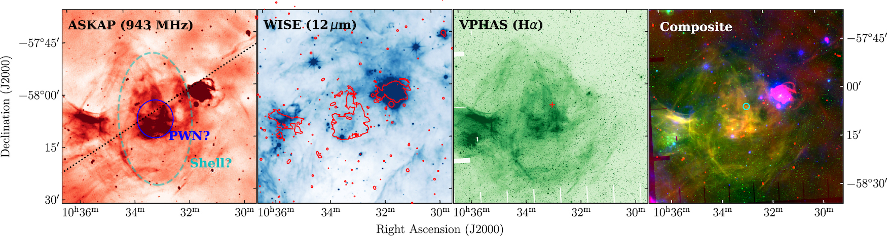
Ziteng Wang (Curtin University) and collaborators used the Australian Square Kilometre Array Pathfinder (ASKAP), a 36-dish radio interferometer, to search for circularly polarized signals from pulsars. In addition to known stars and pulsars, the observations pinpointed a strongly circularly polarized source with no known counterpart at other wavelengths. The team followed up on this promising discovery with the 64-meter Murriyang radio telescope at Parkes Observatory and found a pulsar with a rotation period of 78.72 milliseconds. The pulsar, cataloged as PSR J1032−5804, has an estimated age of 34,600 years, making it relatively young and possibly still associated with a visible supernova remnant. The team found a compact region of emission surrounding the pulsar, but they couldn’t rule out the possibility that the material belongs to unrelated nebulae.

PSR J1032−5804 is notable because its pulses are highly scattered by interstellar gas and dust. Highly scattered pulsar signals are hard to detect because scattering broadens and weakens the signal, especially at lower frequencies where pulsars should be at their brightest. Wang’s team has shown that searching at relatively high frequencies — the team’s observations were made at 3 gigahertz — is a viable way to detect scattered pulsars.

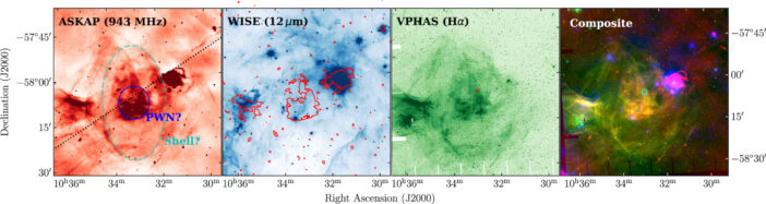
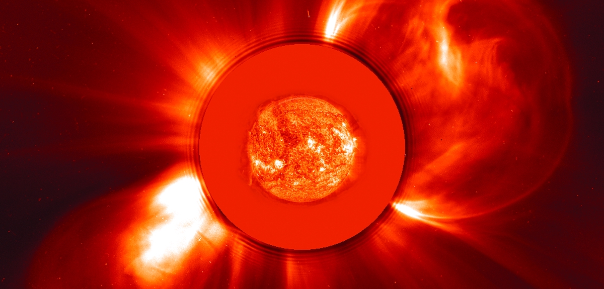
The field surrounding PSR J1032−5804 shown at, from left to right, radio, infrared, and visible wavelengths, as well as a composite of all three. [Wang et al. 2024]

How Do Pulsars Make Their Pulses?

Pulsars may be most famous for their characteristic pulses of radio emission, but the origin of those pulses is still under debate. To understand what powers these radio beacons, researchers use detailed simulations that track the behavior of individual particles to understand how they behave under the exotic conditions present at the surface of a pulsar. To date, localized simulations have been able to produce radio waves from a pulsar’s poles, and global simulations have discerned the source of pulsars’ gamma-ray pulses (10% or so of pulsars produce gamma-ray pulses in addition to radio pulses), but radio pulses have not yet been seen in global simulations.

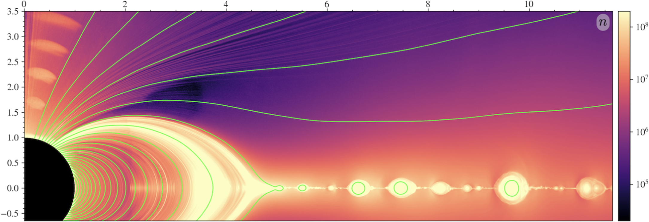
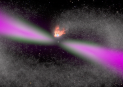
Ashley Bransgrove (Columbia University and Princeton University) and collaborators carried out high-resolution global simulations of a pulsar’s magnetosphere: the region immediately surrounding a pulsar where its strong magnetic field dominates the motion of charged particles. The simulations show how the rapid rotation of the pulsar lofts charged particles from its surface and accelerates them, filling the magnetosphere with gamma rays and a dense sea of electrons and their positively charged counterparts, positrons. Near the pulsar’s poles and farther out in its magnetosphere, gaps form where the electric current is mismatched, and pairs of electrons and positrons are generated in these gaps. When the gaps discharge — think of a spark, or lightning — they excite waves in the plasma and, subsequently, electromagnetic waves. The emitted radiation is similar in frequency and luminosity to observed pulsars, suggesting that electric discharge may generate the radio waves that pulsars are known for.

The team notes that it’s too soon to apply their simulations to observations of individual pulsars, and more work is needed to understand the role of gamma-ray emission, explore the details of electron–positron pair production, and extend the work to pulsars whose spin axes and magnetic axes are misaligned.

plot of simulation output showing magnetic field lines and plasma density

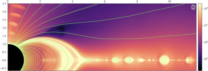
Simulation output showing the magnetic field lines (green curves) and plasma density (background color) in a pulsar’s magnetosphere. [Bransgrove et al. 2023]

How Do Pulsars Interact with Their Surroundings?

map showing the location of the Boomerang within the supernova remnant

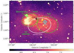
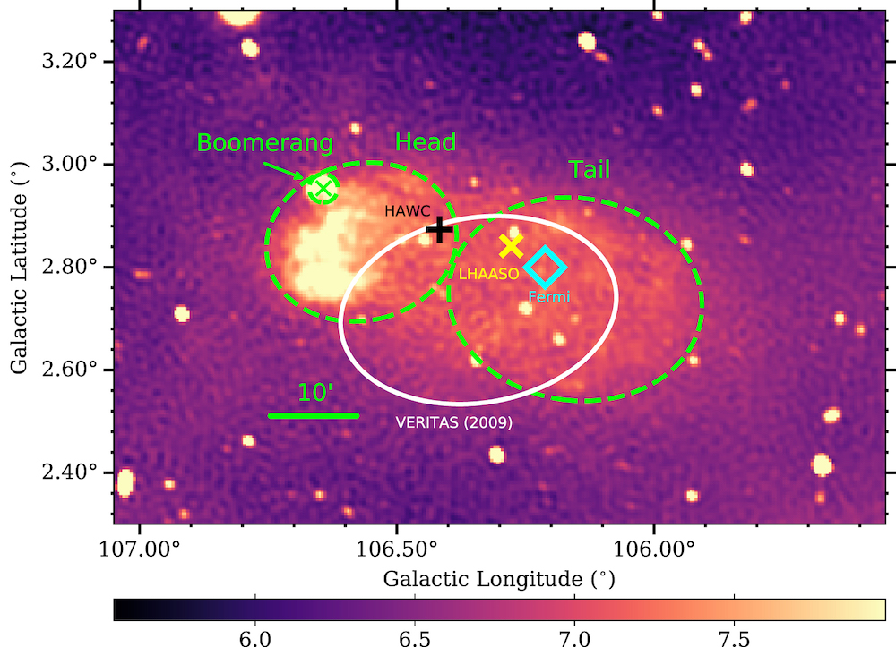
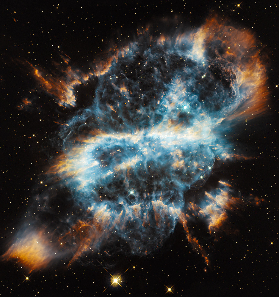
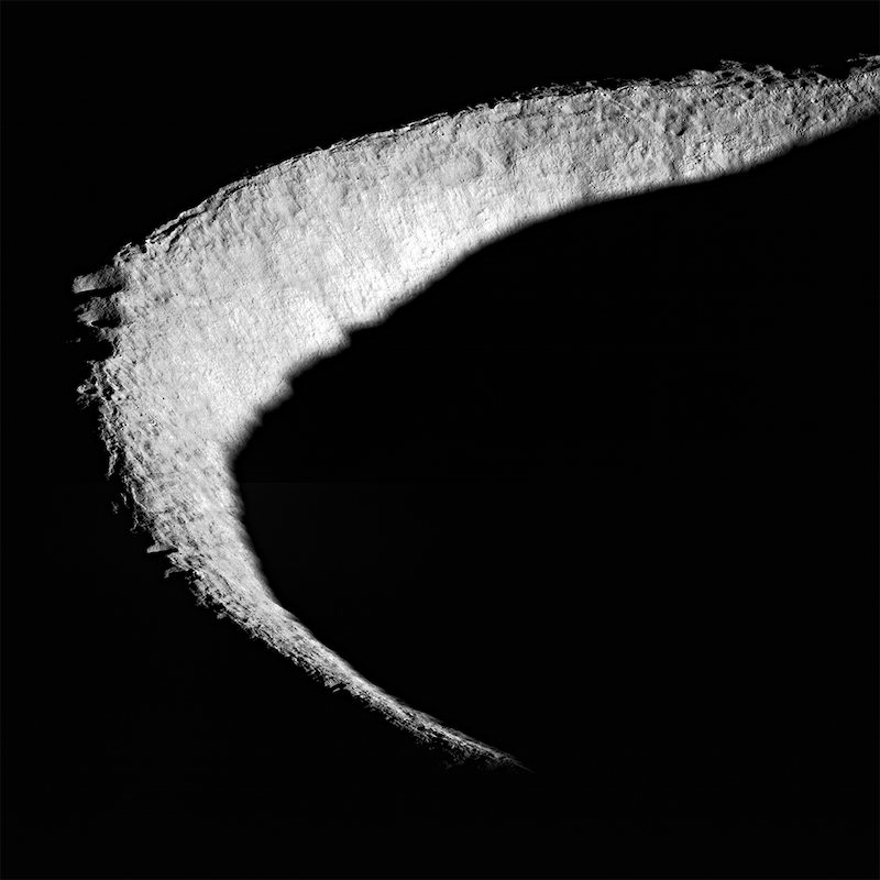
The location of the Boomerang within the supernova remnant surrounding the pulsar PSR J2229+6114. [Pope et al. 2024]

When pulsars are young, they’re swaddled in the gas and dust of their surrounding supernova remnants. This leads young pulsars to create a pulsar wind nebula: a glowing cloud of gas energized by winds of relativistic charged particles streaming off the pulsar. A recent article authored by the Nuclear Spectroscopic Telescope Array (NuSTAR) and Very Energetic Radiation Imaging Telescope Array System (VERITAS) collaborations presents multiwavelength observations of the Boomerang, a 10,000-year-old pulsar wind nebula well known for its complex structure.

The teams combined archival data from radio telescopes and the Chandra X-ray Observatory with newly collected data from NuSTAR, VERITAS, and the Fermi Gamma-ray Space Telescope to probe the nebula’s multiwavelength behavior. These observations revealed that the nebula appears far larger at radio wavelengths than at X-ray wavelengths, a common feature of pulsar wind nebulae due to the difference sources of emission: the nebula’s size at radio wavelengths is set by outflowing particles, while its size at X-ray wavelengths comes from the rate at which electrons lose energy as they spiral around magnetic field lines and emit X-rays. The nebula’s size even varies across X-ray wavelengths, appearing smaller at shorter wavelengths.

Judging from how the nebula’s size changes with wavelength, its overall energy output, and its X-ray emission over the past two decades, the authors provide a new estimate on its distance and magnetic field strength, finding it to be more distant and with a far weaker magnetic field than previously thought. By modeling how the nebula’s energy output may have evolved over time, the team also found that the Boomerang is, well, boomeranging! Roughly 1,000 years ago, a backwards-moving supernova shock wave crashed into the expanding nebula, crushing the nebula and temporarily reversing its expansion. Today, the nebula is re-expanding in the wake of the shock wave, showcasing how pulsars dynamically interact with their surroundings.

Citation

“Discovery of a Young, Highly Scattered Pulsar PSR J1032-5804 with the Australian Square Kilometre Array Pathfinder,” Ziteng Wang et al 2024 ApJ 961 175. doi:10.3847/1538-4357/ad0fe8

“Radio Emission and Electric Gaps in Pulsar Magnetospheres,” Ashley Bransgrove et al 2023 ApJL 958 L9. doi:10.3847/2041-8213/ad0556

“A Multiwavelength Investigation of PSR J2229+6114 and Its Pulsar Wind Nebula in the Radio, X-ray, and Gamma-ray Bands,” I. Pope et al 2024 ApJ 960 75. doi:10.3847/1538-4357/ad0120

A rendering of a planet trailed by a tail of material.

Black widow pulsars are cruel, fascinating beasts that have understandably attracted much attention. Recently, a new set of radio observations has shined light not on the pulsars themselves, but on the properties of their unlucky victims.

Cruel Stars

Black widow pulsars, as their name suggests, easily rank among the deadliest creatures that roam our galaxy. These vicious beasts are a member of the pulsar family, meaning they are dense balls of neutrons formed during the collapse of a massive star. Similarly to a more peaceful (though still quite energetic) subset of their pulsar brethren, they spin so rapidly that they complete one rotation in less than a hundredth of a second. Unlike their docile counterparts, however, each black widow has trapped a low-mass companion into a nearby orbit. These companions, usually a small star or a brown dwarf, feel the full force of the intense radiation spewing from their captors. As the companion helplessly circles the pulsar, this radiation strips material away and peels the object apart. Eventually, the companion meets the same fate as the insolent soldiers who gazed upon forbidden artifacts in Steven Spielberg’s Raiders of the Lost Ark: they melt into nothingness, unable to withstand the heat.

An illustration of a black widow pulsar that includes the tail of the disintegrating companion. [NASA’s Goddard Space Flight Center]

Astronomers have watched one of these monsters named PSR J2051−0827 slowly destroy an unlucky brown dwarf since the late 1990s. Recently, however, their view of this gruesome spectacle improved thanks to the Five-hundred-meter Aperture Spherical radio Telescope (FAST) in China. A team led by S.Q. Wang, Xinjiang Astronomical Observatory, analyzed new observations taken with this facility to inspect the disintegrating brown dwarf in exquisite detail.

An Unwilling Comet

As the doomed brown dwarf completes laps around the pulsar, the material blown off forms a long tail extending behind it, much like a scaled-up comet. This material slightly impedes our view of the system from Earth, and with periodic regularity, it causes different properties of the observed radio emission to shift around. The simplest of these properties is the brightness of the emission: When the densest part of the comet-like tail falls into our line of sight to the pulsar, some low frequencies are blocked entirely, while higher frequencies manage to shine straight through. These “eclipses” have been seen in this system and others in the past, and the range of frequencies blocked can help constrain the environment of the tail.

A series of a line plots, the bottom most of which shows an exponential-looking drop off between the lines mentioned.

Different measured quantities as a function of the brown dwarf’s orbital phase. The bottom plot show the rotation measure: the authors attribute the decrease between the dash-dotted and dashed vertical line to the tail’s magnetic field. [Adapted from Wang et al. 2024]

Besides simple intensity, astronomers can also measure a property known as the rotation measure (RM) of the emission. This slightly abstract quantity measures how the polarization of the emission has changed since it left the pulsar: radiation departs the black widow with a certain polarization, but any magnetized material it encounters along the way to our telescopes on Earth causes that polarization to shift slightly in a way that’s imprinted on the RM.

During the main eclipse, the relatively dense, turbulent material of the tail leaves the polarization scrambled in a way that makes it difficult to measure the RM. However, during the egress of the eclipse when the tail begins to thin out, Wang and collaborators discovered that the RM steadily decreased until it reached its steady, out-of-eclipse value. They infer that this shift is due to a magnetic field in the tail: the material that used to make up the outer atmosphere of the brown dwarf is slightly magnetized with a field strength of about 0.1 Gauss, a little weaker than Earth’s magnetic field at the surface.

Novel, For Now

The researchers note that this is the first time this orbital-phase-dependent change in the RM has been observed, meaning that it’s also the first precise measurement of the magnetic field in the material blown away from black widow’s a companion. However, with FAST now fully operational and proven capable of this kind of measurement, similar observations are likely to follow. We’re likely about to learn much more about the tragic futures of these low-mass companions, and in doing so, more about the pulsars that will bring about about their demise.

Citation

“Change of Rotation Measure during the Eclipse of a Black Widow PSR J2051−0827,” S. Q. Wang et al 2023 ApJ 955 36. doi:10.3847/1538-4357/acea81

illustration of an exoplanet around a white dwarf with a debris disk

JWST has directly imaged what appear to be two giant exoplanets in orbit around white dwarf stars. This discovery has important implications for the fate of giant planets in our solar system as the Sun evolves into a red giant and eventually becomes a white dwarf.

planetary nebula NGC 5189

A planetary nebula appears briefly during the life cycle of most stars, including those like the Sun. Planetary nebulae tend to appear round or elliptical, but they can have dramatically varied shapes, like NGC 5189 shown here. [NASA, ESA, and the Hubble Heritage Team (STScI/AURA)]

The Fate of Most Stars

While brilliant supernova explosions demand our attention when they burst onto the scene, the vast majority of stars will end their lives more quietly, lofting their outer layers into space and forming a glowing planetary nebula that surrounds the star’s exposed core. The core, now a white dwarf containing roughly the mass of the Sun in a sphere roughly the size of Earth, starts out extremely hot and cools slowly over billions of years.

As stars evolve from main-sequence stars to red giants to white dwarfs, it’s clear that close-in planets will meet a fiery fate: as a red giant, the Sun will swell to more than 200 times its current radius, engulfing Mercury, Venus, and possibly Earth. But exactly how the transition affects planets watching things unfold from a distance isn’t yet clear. To learn more, we’ll need to study planets that survived the transformation, and recent observations with JWST may have revealed two planets that fit the bill.

Investigating Metal-Polluted White Dwarfs

Only a handful of planetary-mass objects have been discovered around white dwarfs, but many more are thought to exist; 25–50% of seemingly solo white dwarfs show metals in their spectra, which suggests that they’re collecting cast-off material from unseen planets or asteroids. If giant planets are common around these “metal-polluted” white dwarfs, it would suggest that 1) these planets are able to survive their home star’s red giant phase, and 2) they play a role in gravitationally nudging material toward the white dwarf.

images of two white dwarfs with their candidate planetary companions

The two white dwarfs and their candidate planets. The object in the upper-left corner of the top row of images is a galaxy. [Mullally et al. 2024]

Susan Mullally (Space Telescope Science Institute) and collaborators pointed JWST at four white dwarfs that may harbor planets. These white dwarfs have been shown to contain metals in their atmospheres and are young enough or close enough that their planets would be relatively bright. Even before carefully removing the white dwarfs’ light from the images, Mullally’s team spotted what they were looking for — a possible giant planet around two of the four white dwarfs.

Potential Planets on Outlying Orbits

The observations show a reddish object near two of the white dwarfs. If these objects are indeed planets and the same ages as their host white dwarfs (5.3 and 1.6 billion years old), they likely have masses of 1–7 and 1–2 Jupiter masses, respectively. They’re currently orbiting at estimated distances of 11.47 and 34.62 astronomical units (au), which correspond to orbital distances of 5.3 au and 9.7 au when their host stars were on the main sequence — similar to the present-day orbital distances of Jupiter and Saturn.

comparison of the ages and orbital separations of the two new planet candidates with the giant planets in our solar system and planetary-mass objects previously discovered through direct imaging

A comparison of the ages and orbital separations of the two new planet candidates (red triangles), the four giant planets in our solar system (blue stars), and objects with masses less than 12 Jupiter masses discovered previously through direct imaging (black circles). Click to enlarge. [Mullally et al. 2024]

While the objects appear to be associated with the white dwarfs, it’s not impossible for them to instead be small photobombing objects within our solar system or distant, reddish galaxies meandering in the background. The authors pin the likelihood of their detections being a false positive at 1 in 3,000.

If future JWST observations show that these white dwarfs and their candidate planetary companions march across the sky in step, it will mark the first direct imaging detection of planets similar to the giant planets in our solar system in age, mass, and orbital distance. More than that, it will provide evidence that widely separated planets survive their host stars ballooning into red giants, and that giant planets around white dwarfs are common and help their hosts accrete metal-rich material.

Citation

“JWST Directly Images Giant Planet Candidates Around Two Metal-Polluted White Dwarf Stars,” Susan E. Mullally et al 2024 ApJL 962 L32. doi:10.3847/2041-8213/ad2348

photograph of Earth

The chaotic interactions between solar system bodies prevent us from knowing Earth’s precise orbit billions of years in the past or future. New research shows that passing stars introduce even more uncertainty, shortening the time out to which we can reliably predict Earth’s past orbit by 10%.

Uncertain Future, Uncertain Past

a map of the solar system planets and 18,000 solar system asteroids

A map showing the positions of the planets and 18,000 asteroids on New Year’s Eve in 1999. Click for the high-resolution version of this image. [Eleanor Lutz; CC BY-NC-ND 4.0]

Though the solar system may seem stable and predictable, with the planets moving calmly along well-defined orbits, this stability may only be temporary. Planets and asteroids gravitationally nudge one another, introducing an element of chaos into the calm and making it possible — though improbable — that one or more planets in our solar system will be ejected or destroyed in the next 5 billion years.

This chaotic element doesn’t just introduce uncertainty into the future behavior of the planets. It also means we can’t look infinitely far into their past motions, either. For Earth, the limit seems to lie around 60–70 million years ago, meaning that we cannot extrapolate Earth’s orbital history beyond that point. Because changes in Earth’s orbit influence our planet’s climate, researchers interpreting the ancient climate record contained in ice cores and sediment consider the behavior of Earth’s past orbit, and it’s critical for them to know how far back our orbital simulations are reliable.

Previous studies have focused on how planets and asteroids affect simulations of Earth’s past orbit. But the solar system doesn’t exist in a vacuum (metaphorically speaking) — could passing stars affect our ability to study Earth’s orbital history as well?

Chaos Caused by Passing Stars

In a research article published today, Nathan Kaib (Planetary Science Institute and University of Oklahoma) and Sean Raymond (National Centre for Scientific Research, France; University of Bordeaux) used numerical simulations to understand how passing stars impact our ability to trace back Earth’s orbit. Kaib and Raymond added a tiny amount of scatter in the positions of the planets and large asteroids and allowed the system to evolve backwards over 150 million years of simulation time.

plot showing the standard deviation of Earth's orbital eccentricity over time

The standard deviation of Earth’s orbital eccentricity as a function of time in the past. [Kaib & Raymond 2024]

Some of the simulations contained stars placed at random positions about 3.4 light-years from the Sun and given random velocities. (Technically, all of the simulations contained passing stars, but in the star-free runs the stars’ masses were set to minuscule values. This prevents the results from depending on the computational methods being used rather than the presence of the stars.) By marking the moment at which Earth’s orbital eccentricity, or how circular its orbit is, diverged by more than 10%, the authors determined how far back their simulations of Earth’s orbit were reliable.

Close Encounters of the Stellar Kind

plot of the change in Earth's orbital eccentricity over time, showing the effects of a close stellar encounter

The change in Earth’s orbital eccentricity, showing the effects of an HD 7977-like encounter at a time of 10 million years. Click to enlarge. [Adapted from Kaib & Raymond 2024]

Kaib and Raymond found that passing stars interfere with our ability to trace back Earth’s orbit, shortening the time we can reliably look back by about 10%. The simulations suggest that stars act on Earth by nudging the giant planets, which then nudge Earth; when the giant planets were removed from the simulation, passing stars had little effect.

To look more closely at a specific event, Kaib and Raymond considered the star HD 7977. HD 7977 currently sits about 250 light-years away, but its trajectory suggests that it passed within about 13,200 astronomical units (au) of our solar system 2.8 million years ago, making it possibly the closest recent stellar encounter. The team showed that the star’s passage likely didn’t impact Earth’s orbit much, unless the star came as close as the data allow — there’s a 5% chance that the star came within 3,900 au.

If HD 7977 did approach the solar system so closely, the encounter may have introduced a large amount of uncertainty into simulations of Earth’s past orbit. This allows for a broader range of past orbital eccentricities, opening up new possibilities to consider for Earth’s orbital and climatic past.

Citation

“Passing Stars as an Important Driver of Paleoclimate and the Solar System’s Orbital Evolution,” Nathan A. Kaib and Sean N. Raymond 2024 ApJL 962 L28. doi:10.3847/2041-8213/ad24fb

photograph of craters on the Moon's north pole

On Earth, rocks and soil are weathered by wind and water, but what weathers surfaces on the Moon? New research investigates how ice might alter lunar soil in permanently shadowed lunar craters.

The Importance of Lunar Soil

photograph of the sunlit edge of a crater on the Moon

Photograph of the sunlit rim of Shackleton crater, a crater at the Moon’s south pole. The interior of this crater never receives direct sunlight. [NASA/GSFC/Arizona State University]

The Moon is blanketed in a layer of material called regolith, made up of fragments of rock, soft lunar soil, and fines: particles less than 2 microns across (1 micron = 10-6 meter). Apollo-era astronauts encountered fines during moonwalks; the fines clung relentlessly to every surface and caused sneezing and sore throats when brought in to the lunar module. Lunar fines aren’t just annoying — studies using simulated lunar material show that fines can damage lung cells and DNA.

NASA’s upcoming Artemis missions will bring astronauts to the lunar south pole, which is dotted with steep-sided craters that lie in permanent shadow. Because some of these craters are thought to harbor water ice, it’s important to know if the ice is likely to weather the lunar surface material, creating an abundance of harmful and irritating fines.

A Lunar Experiment on Earth

Autumn Shackelford (University of Central Florida) and collaborators examined how lunar regolith might be weathered by water ice. If a tiny bit of liquid water seeps into fine cracks in lunar surface particles, the expansion of the water as it freezes will widen the cracks. The mechanical stress caused by this expansion may cause the crack system to grow, potentially reshaping the particle.

close-up image of particles in one of the samples

An image of a sample that contained 30% water by weight and was frozen for 6 months. The numbering and outlines reflect the counting and characterization of individual particles and clumps of particles. Click to enlarge. [Shackelford et al. 2024]

To understand how water ice plays a role in the weathering process, Shackelford’s team mixed samples of simulated lunar soil with water and placed the samples in a freezer. Half of the samples contained minerals similar to the lunar highlands (the lighter regions of the Moon’s surface), while the other half were similar to the lunar “seas,” or maria (the darker regions of the Moon’s surface).

The team varied the amount of water added to the samples from no water — the control samples — to 30% water by weight, and left the samples in a freezer for 1, 3, or 6 months. After the samples finished hibernating, the team characterized the size and shape of the particles, counted the number of fine particles, and took spectra to search for possible spectral changes.

Water Weathering

Plots of the number of fines per particle imaged

The number of fines per particle, as a function of time spent in the freezer, amount of water, and type of particle. Click to enlarge. [Shackelford et al. 2024]

Contact with water ice changed the shapes and sizes of the simulated lunar particles, and the changes were dependent upon the amount of water, the time spent in the freezer, and whether the sample was similar to the lunar highlands or the lunar maria. Crucially, the amount of fine particulate matter — the material that was so perplexing during the Apollo missions — generally increased with both water content and time spent in the freezer. The lunar mare samples produced more fine particles than the lunar highlands samples in all cases, showing that composition plays an important role. Curiously, while the highlands simulant showed changes in its spectrum in the 5–22.5-micron range after exposure to ice, the mare samples showed no spectral changes.

With humans potentially exploring lunar regions where water ice lingers in shadowy craters, this work provides an important first look at how ice plays a role in producing fine particles. Future astronauts, take heed!

Citation

“Morphological and Spectral Characterization of Lunar Regolith Breakdown Due to Water Ice,” A. Shackelford et al 2024 Planet. Sci. J. 5 1. doi:10.3847/PSJ/ad0041

extreme-ultraviolet image of solar coronal loops

Many models of the Sun’s upper atmosphere, or corona, use magnetohydrodynamics, in which collections of particles are assumed to behave like an electrically conducting fluid. A recent research article explores how sensitive magnetohydrodynamics models are to the conditions they start with.

A Powerful Modeling Tool

image of the Sun releasing two coronal mass ejections

Two coronal mass ejections launched from the Sun in November 2000, as seen by the Solar and Heliospheric Observatory. [ESA/NASA/SOHO]

Magnetohydrodynamics simulations are a solar modeler’s bread and butter. These powerful simulations can be applied to everything from the slow shifting of the solar magnetic field as the Sun proceeds through its 11-year solar activity cycle to the rapid release of magnetic energy in solar flares or coronal mass ejections.

With so many ways to implement these models, it’s worth taking the time to consider how choices of model parameters affect the outcome. In other words, how much does what you get out depend on what you put in?

Testing Model Memory

To begin to address this question, Graham Barnes (NorthWest Research Associates) and collaborators studied the impact of initial conditions on magnetohydrodynamics simulations of the solar corona driven by electric fields. Just as the term suggests, initial conditions refer to the state of the model just before the modelers press go. For example, modelers might define the initial strength and direction of magnetic and electric fields and the density, temperature, and motion of the particles.

After a simulation begins, it will often undergo an adjustment period in which the initial quantities “relax” into a steady state. Once this steady state is reached, the model can be “driven,” such as by applying a force to the base of the corona, to study how the system changes over time. Barnes’s team sought to understand whether a model’s “memory” of the initial conditions persists through this relaxation phase. If the initial conditions are washed out during the relaxation phase, that means that any reasonable choice of parameters will do — but if the models retain a clear memory, researchers must choose their initial conditions more carefully.

Relating Relaxed Output to Initial Input

plots of the vertical magnetic field of two active regions

The two active regions used in this study. The greyscale shows the strength of the vertical component of the magnetic field. Click to enlarge. [Barnes et al. 2024]

The team focused on the initial state of the magnetic field. They modeled two solar active regions — areas with particularly strong and complex magnetic fields — using data from the Solar Dynamics Observatory’s Helioseismic and Magnetic Imager, which measures the vertical component of the solar magnetic field. They used three methods to derive the initial strength and direction of the magnetic field from the data: a commonly used potential field, a slightly more realistic representation of the corona’s magnetic field (the nonlinear force-free field), and a purely vertical field. Then, Barnes’s team allowed the simulations to relax by letting the magnetic field evolve over time while reverting other quantities, like the density of the solar plasma, back to their initial values at each time step.

comparison of initial conditions and steady state outcomes for three choices of initial conditions

Initial conditions (top row) and relaxed state (bottom row) for the modeled magnetic field of one of the active regions. This shows that the relaxed state is largely insensitive to the initial state when comparing potential field, nonlinear force-free field, and vertical field initial conditions. Click to enlarge. [Adapted from Barnes et al. 2024]

Barnes and collaborators found that the initial magnetic field conditions had little impact on the relaxed state of the magnetic field — the simple vertical magnetic field and the more realistic fields had remarkably similar outcomes. What differences did arise tended to show up at the borders of the simulation, where edge effects and boundary conditions play a larger role.

With models appearing to lack a clear memory of the conditions they started with, this work suggests that any reasonable initial magnetic field can be used for electric-field-driven models. More work is needed to understand if this result holds for other types of magnetohydrodynamics models, such as velocity-driven models.

Citation

“Are Electric-Field-Driven Magnetohydrodynamic Simulations of the Solar Corona Sensitive to the Initial Condition?” Graham Barnes et al 2024 ApJ 960 102. doi:10.3847/1538-4357/ad10a7

1 24 25 26 27 28 119