Could Flaring Stars Change Our Views of Their Planets?
As the exoplanet count continues to increase, we are making progressively more measurements of exoplanets’ outer atmospheres through spectroscopy. A new study, however, reveals that these measurements may be influenced by the planets’ hosts.
Spectra From Transits
Exoplanet spectra taken as they transit their hosts can tell us about the chemical compositions of their atmospheres. Detailed spectroscopic measurements of planet atmospheres should become even more common with the next generation of missions, such as the James Webb Space Telescope (JWST), or Planetary Transits and Oscillations of Stars (PLATO).
But is the spectrum that we measure in the brief moment of a planet’s transit necessarily representative of its spectrum all of the time? A team of scientists led by Olivia Venot (University of Leuven in Belgium) argue that it might not be, due to the influence of the planet’s stellar host.
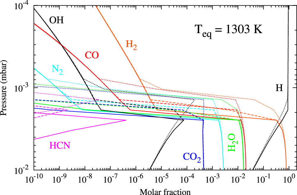
Atmospheric composition of a planet before flare impacts (dotted lines), during the steady state reached after a flare impact (dashed lines), and during the steady state reached after a second flare impact (solid lines). [Venot et al. 2016]
Modeling Atmospheres
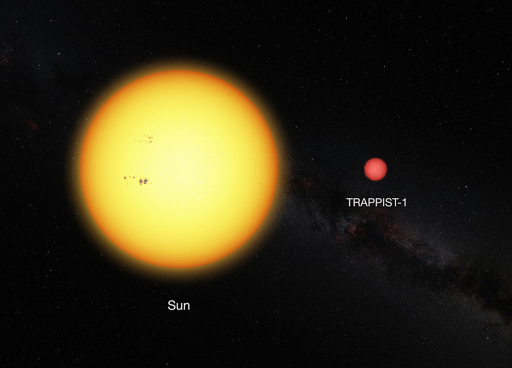
Venot and collaborators set out to test the effect of stellar flares on exoplanet atmospheres by modeling the atmospheres of two hypothetical planets orbiting the star AD Leo — an active and flaring M dwarf located roughly 16 light-years away — at two different distances. The team then examined what happened to the atmospheres, and to the resulting spectra that we would observe, when they were hit with a stellar flare typical of AD Leo.
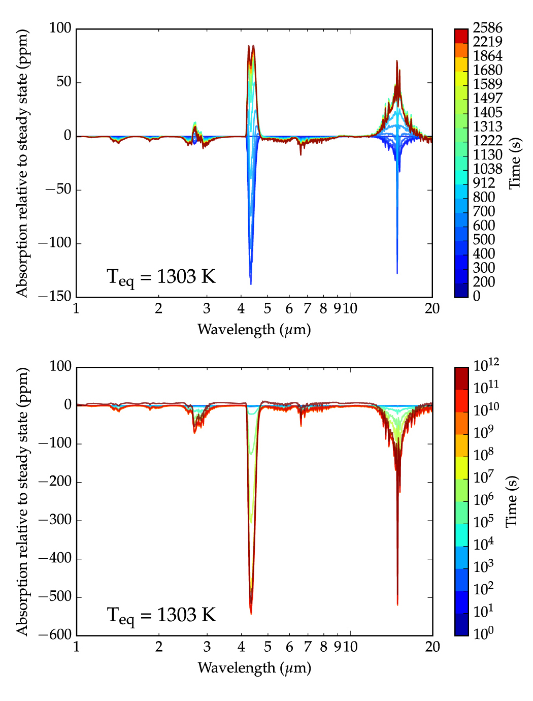
The difference in relative absorption between the initial steady-state and the instantaneous transmission spectra, obtained during the different phases of the flare. The left plot examines the impulsive and gradual phases, when the flare first impacts and then starts to pass. The peak photon flux occurs at 912 seconds. The right plot examines the return to a steady state over 1012 seconds, or roughly ~30,000 years. [Adapted from Venot et al. 2016]
Permanent Impact
In addition to demonstrating that a planet’s atmospheric composition changes during and immediately after a flare impact, Venot and collaborators show that the chemical alteration isn’t temporary: the planet’s atmosphere doesn’t fully return to its original state after the flare passes. Instead, the authors find that it settles to a new steady-state composition that can be significantly different from the pre-flare composition.
For a planet that is repeatedly hit by stellar flares, therefore, its atmospheric composition never actually settles to a steady state. Instead it is continually and permanently modified by its host’s activity.
Venot and collaborators demonstrate that the variations of planetary spectra due to stellar flares should be easily detectable by future missions like JWST. We must therefore be careful about the conclusions we draw about planetary atmospheres from measurements of their spectra.
Citation
Olivia Venot et al 2016 ApJ 830 77. doi:10.3847/0004-637X/830/2/77

![Properties of the galaxies included in the authors’ sample. Left: redshifts for galaxy pairs. Right: Number of satellite galaxies around hosts. [Adapted from Libeskind et al. 2016]](https://aasnova.org/wp-content/uploads/2016/12/fig22.jpg)
![Probability that satellites are located at an angle of θ degrees from the direction pointing toward the other galaxy in the pair. There are more satellites found in the space between the pair than predicted by a uniform distribution. [Libeskind et al. 2016]](https://aasnova.org/wp-content/uploads/2016/12/fig31.jpg)


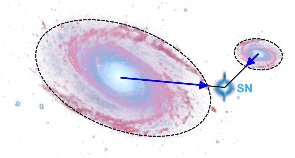
![The matching algorithm’s accuracy (“purity”) as a function of the true supernova-host separation, the supernova redshift, the true host’s brightness, and the true host’s size. [Gupta et al. 2016]](https://aasnova.org/wp-content/uploads/2016/11/fig44.jpg)

![The evolution with redshift the authors find for the mean X-ray background intensities. Each curve represents a different observed X-ray energy (and the total X-ray background is given by the sum of the curves). The two panels show results from two different calculation methods. [Xu et al. 2016]](https://aasnova.org/wp-content/uploads/2016/11/fig36.jpg)