Astrobites RSS

Hubble Space Telescope infrared image of the host galaxy of FRB 180916.

Editor’s note: Astrobites is a graduate-student-run organization that digests astrophysical literature for undergraduate students. As part of the partnership between the AAS and astrobites, we occasionally repost astrobites content here at AAS Nova. We hope you enjoy this post from astrobites; the original can be viewed at astrobites.org.

Title: A High-Resolution View of Fast Radio Burst Host Environments
Authors: Alexandra G. Mannings et al.
First Author’s Institution: University of California, Santa Cruz
Status: Submitted to ApJ

First discovered in 2007, fast radio bursts (FRBs) have been the talk of the town for the last few years. As their name suggests, FRB sources emit very fast (millisecond-long) bursts of radiation at radio frequencies. Due to their very high dispersion measures (DMs), we know that FRBs are typically located in galaxies outside of the Milky Way, although the first galactic FRB was detected in March 2020. While the majority of FRBs are one-off events, some FRBs repeat, and two even repeat periodically! Even with the huge effort to study FRBs over the last few years, however, we still have much to learn about these objects.

In particular, while hundreds of FRBs have been discovered, we have only localized about a dozen FRBs to their respective host galaxies. Localizing FRBs is very important for auxiliary science, such as the missing baryon problem, and for determining what produces FRBs. By comparing FRB host environments with the hosts of other transients, we can hopefully determine whether FRBs might come from similar origins. This is what today’s authors explore!

Hubble for the Win!

The authors use infrared (IR) and ultraviolet (UV) observations from the Hubble Space Telescope to study the host galaxies of eight different FRBs. Six of these observations are newly presented, while the host galaxy of the infamous FRB 121102 (the first repeating FRB) and FRB 180916 (the first periodic FRB) were reported in previous studies.

So What Is Cooking for These Eight FRBs?

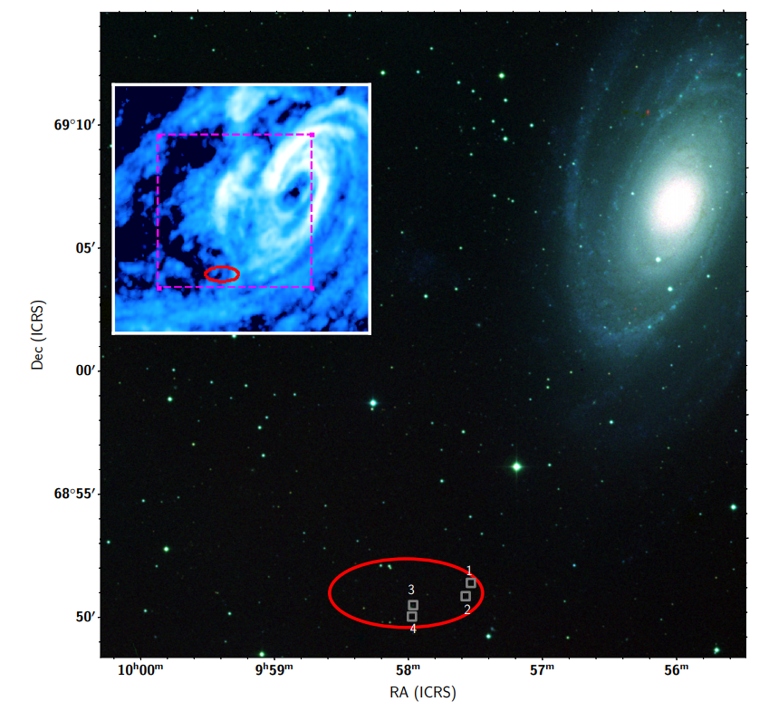
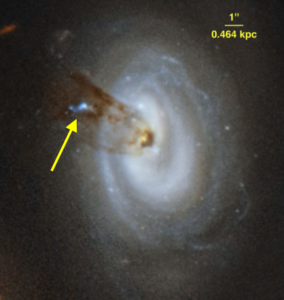
First, the authors locate the FRBs within their host galaxies. Of the eight FRBs, five are located within spiral galaxies as shown below in Figure 1. This is not unexpected, as ~60% of the observed galaxies in our universe are spiral galaxies. While they are located within the spiral arms of their hosts, the five FRBs are not actually located at the brightest points of the spiral arms (but note that they have huge error regions!).

Hubble Space Telescope images for each of the host galaxies. FRB 180916, FRB 191001, FRB 190608, FRB 190714, and FRB 180924 all reside in spiral galaxies.

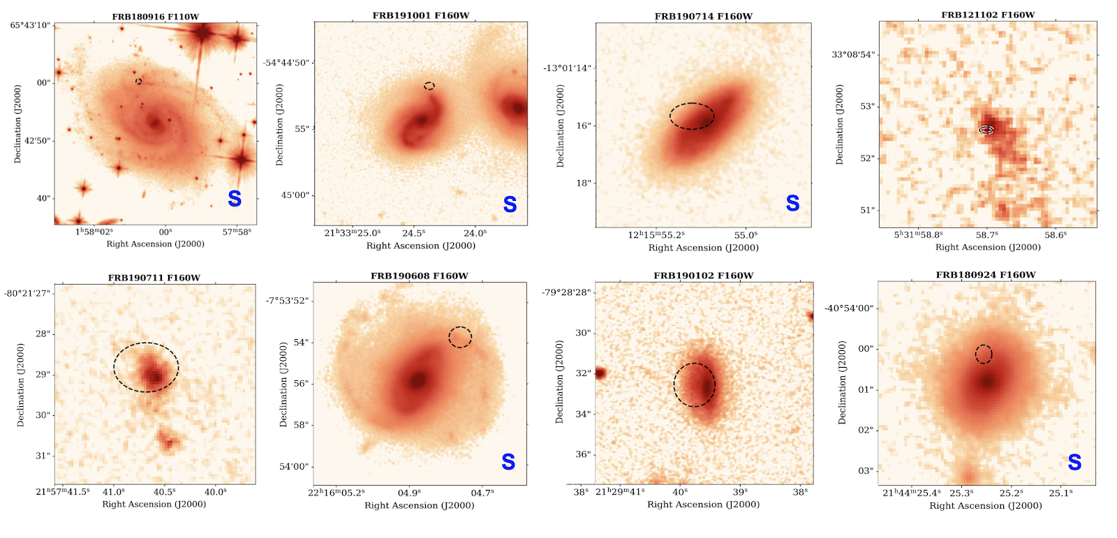
Figure 1: Host galaxy images for each of the FRBs with the FRB location circled. The FRBs that reside in spiral arms are labelled using a blue “S.” [Mannings et al. 2021]

The authors are also able to convert the UV light at the position of the FRB to the star formation rate density at this position, and the IR light at the position of the FRB to the stellar mass surface density at this location. As shown below in Figure 2, only FRB 121102 and FRB 180916 lie in areas with a lot of star formation (and the star formation rate for FRB 180916 is an upper limit). The other FRBs tend to lie in more moderate, although slightly higher than average, regions. This is a bit surprising as young magnetars, a very popular origin for FRBs, are typically located very close to points of high star formation.

There is almost a perfect 1:1 correlation between the stellar mass surface density at the location of the FRB and the average for the FRB’s galaxy, suggesting that FRBs lie in typical surface mass density regions within their host galaxies.

two plots describing properties of the environment around 8 localized FRBs.

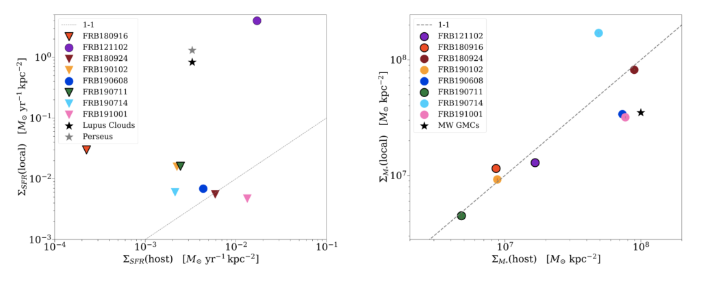
Figure 2: Left: Comparison between the star formation rate density for different FRBs as compared with the average for the host. There is no clear relation between the two, but we note that many of the observations are upper limits (indicated with triangles). Right: Comparison between the stellar mass surface density for different FRBs as compared with the average for the host. There is almost a perfect 1:1 relation between the two. [Mannings et al. 2021]

The authors also use the properties of the FRBs within their host galaxies to try to identify (or rule out) possible mechanisms for the origins of FRBs. In particular, they focus on five properties:

  1. The distance between the FRB and the center of the host galaxy, i.e., the radial offset.
  2. The distance between the FRB and the center of the host galaxy after normalizing by the size of the galaxy, i.e., the normalized radial offset.
  3. The brightness of the galaxy at the location of the FRB as compared to the brightness throughout the galaxy in the UV band. The UV light can be used as a proxy for star formation within a galaxy.
  4. The brightness of the galaxy at the location of the FRB as compared to the brightness throughout the galaxy in the IR band. The IR light can be used as a proxy for stellar mass within the host.
  5. The amount of light within the galaxy that is interior to the FRB’s location, known as the enclosed flux.

The authors compare these properties of FRBs within their hosts to that of six different transient phenomena: long duration gamma-ray bursts (LGRBs) short-duration gamma-ray bursts (SGRBs), Ca-rich transients, Type Ia supernovae (Type Ia SNe), core-collapse SNe (CCSNe), and super-luminous SNe (SLSNe). While it can be a bit difficult to remember all of these different transients, they can generally be lumped into three different categories: 1. Massive star explosions (LGRBs, CCSNe, SLSNE) 2. Explosions involving older stellars objects such as neutron star mergers (SGRBs) or white dwarfs (Type Ia SNe), and 3. Objects with unknown origins (Ca-rich transients).

From their comparisons, the authors find that the properties of LGRBs, SGRBs, SLSNe and Ca-rich transients are inconsistent with those of FRBs. The table below indicates which properties are inconsistent for each of these transients (marked with X). The authors cannot rule out CCSNe and Type Ia SNE as being associated with FRBs. This is similar to another recent result that finds FRBs are consistent with CCSNe (and hence magnetars born from CCSNe) but different from this result that finds it unlikely that Type Ia SNe are associated with every FRB.

LGRBs SGRBs Type Ia SNe CCSNe SLSNe Ca-rich transients
Radial Offset X X
Normalized Radial Offset X X
Brightness in UV X X
Brightness in IR X X


For the fifth property, the enclosed flux, the authors don’t compare the distribution from the FRBs to that of the other transients. Instead, they only conclude that the FRBs appear to trace the distribution of light within their host galaxies.

So Where Does This Leave Us? 

If there is one key transient associated with FRBs, then this work suggests that it is not LGRBs, SGRBs, SLSNe, or Ca-rich transients. However, there is one very important caveat to the authors’ work, which is that they group repeating and non-repeating FRBs together in their sample. So it is possible that there is not just one but multiple mechanisms responsible for the FRBs within their sample. Thus, the mystery of what produces FRBs continues…

Original astrobite edited by Viraj Karambelkar.

About the author, Alice Curtin:

I’m a second year MsC student at McGill University studying Fast Radio Burts and pulsars using the Canadian Hydrogen Mapping Experiment (CHIME). My work mainly focuses on characterizing radio frequency interference, investigating multi-wavelength counterparts to FRBs, and using pulsars as calibrators of future instruments. When not doing research, I typically find myself teaching physics to elementary school students, spending time with friends, or doing something active outside.

Active Galactic Nucleus

Editor’s note: Astrobites is a graduate-student-run organization that digests astrophysical literature for undergraduate students. As part of the partnership between the AAS and astrobites, we occasionally repost astrobites content here at AAS Nova. We hope you enjoy this post from astrobites; the original can be viewed at astrobites.org.

Title: The Landscape of Galaxies Harboring Changing-Look Active Galactic Nuclei in the Local Universe
Authors: Sierra A. Dodd et al.
First Author’s Institution: University of California, Santa Cruz
Status: Published in ApJL

As we grow older and learn more about ourselves, we sometimes think about changing our appearance: a new hairstyle, clothes, or maybe even a tattoo! Active galactic nuclei (AGN) are, in this respect, no different. Over the course of a galaxy’s lifetime it will accrete gas and dust that will make its way to the centre, where its supermassive black hole (SMBH) resides. As the SMBH feeds on this material, it will emit huge amounts of radiation and become an AGN. However, certain conditions can cause disruptions in the AGN’s gas supply. Whilst the cause of these disruptions is unclear, we can see the effects in the AGN’s changing spectrum. Either they “turn on” as broad optical emission lines emerge or “turn off” as those lines disappear. Today’s authors are interested in identifying what kind of galaxies host these changing-look AGN (CL-AGN) to try to isolate the conditions that might trigger these changes.

Constructing the AGN Lookbook

Identifying CL-AGN involves a comparison between two sets of spectra of the same galaxy taken at two different times to find the changes in the broad emission lines. Different studies will approach this task in their own way but are ultimately following this principle. This is true for all identification techniques, but CL-AGN have only been identified as a phenomenon relatively recently, so very few have been found. To produce today’s sample of 17 CL-AGN, the authors have had to combine detections from three different studies that follow this broad approach but with their own unique characteristics. So, what one study calls a CL-AGN might be slightly different from another. In addition, all but two of these detections are turn-on AGN. The authors argue that the lack of turn-off AGN is due to the relative abundance of quiescent galaxies in the nearby universe. Within these galaxies, it is much easier to see the emergence of broad emission lines. As a result, their sample may not be particularly representative of the underlying CL-AGN population, but the authors are very forthcoming about these issues and have shown care in constructing their sample.

Their comparison sample is a set of 500,000 local galaxies with measured stellar masses, star formation rates and numerous other spectral properties. Most of these quantities are measured across the whole galaxy and are also broken down into bulge and disk components. These data, mostly drawn from the SDSS, will allow today’s authors to place the CL-AGN within the wider galaxy population and isolate the conditions that trigger this change.

Plot showing host galaxy distributions.

Figure 1: Distribution of host galaxies’ star formation rates and stellar masses. Blue circles show the distribution of CL-AGN compared to the underlying comparison galaxies (grey contours). Dashed lines indicate different star formation classifications: green-valley galaxies lie between the dashed blue and orange lines. [Dodd et al. 2021]

Results

From their analysis, we can determine three key consistencies about the preferences of CL-AGN. Figure 1 shows that the CL-AGN are all consistent, within errors, of being hosted in green-valley galaxies. These are a rarer form of galaxy that lie in between the blue, actively star-forming galaxies and their red and dead counterparts. Green-valley galaxies are believed have recently undergone a burst of extreme star formation, possibly implying the presence of large amount of cold gas at the centre which could fuel the mostly turn-on activity seen in this sample.

Plot of galactic asymmetry vs. SMBH mass

Figure 2: Asymmetry of the host galaxy against SMBH mass. Blue circles show the tight distribution of CL-AGN compared to the underlying comparison galaxy distribution (grey contours) and merging galaxies (yellow diamonds). [Dodd et al. 2021]

Gas is often thought to be driven into galaxies through mergers, however figure 2 shows us that CL-AGN are extremely centrally concentrated, especially when compared to the shapes of merging galaxies. In addition, we see that the CL-AGN asymmetry range is much tighter than the wider galaxy population. To explore this idea further, the authors then compare the galaxies’ Sersic indices. This is a measure of the steepness of the galaxy light profile, with larger numbers indicating that stellar light is more centrally concentrated. Figure 3 shows us that the CL-AGN have much higher Sersic Indices than the galaxy population at large. Thus, the authors argue that CL-AGN preferentially reside in very symmetric and centrally concentrated galaxies.

Plot of galaxy concentration vs. SMBH mass

Figure 3: Sersic index (indicating the concentration of galaxy light) against SMBH mass. Both the squares and stars show how CL-AGN are distributed compared to the underlying comparison galaxy distribution (grey contours). [Dodd et al. 2021]

CL-AGN are a relatively novel phenomenon, and working with a sample constructed from multiple different studies may introduce some selection-based uncertainties. The authors admit that their sample may not be perfectly representative of the CL-AGN population, but despite this, they have found a fairly consistent set of properties. Their results imply that CL-AGN in the nearby universe most likely turn on when there is an abundant supply of cold gas and a high concentration of stellar mass in the central region of the host galaxy. Whilst the exact nature of the disruption is still a puzzle, these results will help focus future searches. With a better idea of where to look, strategies can be created that increase the sample of CL-AGNs and help us better understand what causes these transitions to occur.

Original astrobite edited by Alison Crisp.

About the author, Keir Birchall:

Keir is a PhD student studying methods to identify AGN in various populations of galaxies to see what affects their incidence. When not doing science, he can be found behind the lens of a film camera or listening to the strangest music possible.

Illustration of a long, thin, rocky body in the foreground against a backdrop of the galaxy.

Editor’s note: Astrobites is a graduate-student-run organization that digests astrophysical literature for undergraduate students. As part of the partnership between the AAS and astrobites, we occasionally repost astrobites content here at AAS Nova. We hope you enjoy this post from astrobites; the original can be viewed at astrobites.org.

Title: Interstellar Objects in the Solar System: 1. Isotropic Kinematics from the Gaia Early Data Release 3
Authors: T. Marshall Eubanks, Andreas M. Hein, Manasvi Lingam et al.
First Author’s Institution: Space Initiatives Inc.
Status: Submitted to AJ

Comet 2I/Borisov

Hubble image of comet 2I/Borisov, captured just after the comet passed perihelion in December 2019. [NASA/ESA/D. Jewitt (UCLA)]

Three and a half years ago, astronomers discovered something in our solar system that had never been seen before: an object from another star system! Discovered by observatories in Hawaiʻi, this object (illustrated above) was given the name ʻOumuamua, which, in the Hawaiian language, roughly translates to “the first distant messenger.” Two years later, astronomers repeated this feat and discovered yet another interstellar object (ISO) — this one more cometary in appearance. This object was named after its discoverer, Borisov. These types of objects were expected to exist but eluded discovery until just now. So where do these objects actually come from? And how often should we expect to find them, now that we know they’re out there? We explore these questions in today’s astrobite.

An Elegant and Simple Model

The authors address these questions by calculating the “differential arrival rate” (Γ) of interstellar objects. Γ is defined as the number of objects that will pass within a given distance of the Sun every year, as a function of their velocity and perihelion (distance of closest approach to the Sun). Γ is the product of three numbers:

  1. the number density of ISOs (the number of ISOs per unit volume),
  2. the volume sampling rate of ISOs with a certain velocity and perihelion (the rate that a given volume samples ISOs of a certain type), and
  3. the probability distribution function of ISO velocities (the probability of an ISO having a particular velocity).

The first order of business is to calculate the number density of ISOs. For this, the authors turn to previous work, where astronomers used the discovery of ʻOumuamua to place a limit on the number of ISOs within a given volume. This estimate uses the detection rate, i.e., how many such objects are detected per year, divided by the amount of volume that the PanSTARRS observatory surveys per year (PanSTARRS was the first survey to detect ʻOumuamua). Even more time has passed since ʻOumuamua was discovered, and since the quality of surveys has improved as well, this work assumes there may be around half as many ISOs per unit volume as previously predicted.

Calculating the volume sampling rate is a bit more complicated, though it is conceptually straightforward. The amount of volume sampled at a given perihelion is just the cross sectional area enclosed by the perihelion multiplied by the velocity of an ISO (area * velocity = volume / time). However, it is imperative to account for “gravitational focusing,” the phenomenon whereby the Sun’s gravity alters the trajectories of smaller bodies passing through the solar system. The basic idea is that objects moving more slowly will be even more likely to be “focused” towards the Sun on their orbit, thus increasing the volume sampling rate for these types of objects. Nonetheless, this calculation only requires the assumption of a typical perihelion.

The last piece of the puzzle is to determine the probability distribution function of ISO velocities. This is the most difficult of the three necessary ingredients to obtain, and for this, we must consult the stars.

Consulting the Stars to Learn about Interstellar Objects

To recap, the authors want to calculate the differential arrival rate, Γ, of ISOs, or how many ISOs arrive in the solar system per unit time. To do this, they need to know their number density, the rate at which a given volume interacts with ISOs with a given velocity, and the probability of finding ISOs with that speed. Above we outlined how the authors determine the first two. However, if we have only ever discovered two ISOs (which are substantially different from each other), how can we possibly determine this last crucial ingredient, the probability distribution function of ISO velocities?

Here the authors make a basic assumption: the velocity distribution of ISOs relative to the solar system is probably similar to the velocity distribution of the host stars from which they originate. It is true that some objects may be kicked from their star systems at extreme velocities, but most are thought to exit with relatively low ejection velocities. This means all we need to do is measure the three-dimensional motion of a representative sample of stars near our solar system. Thankfully, the Gaia spacecraft, launched in 2013, has measured the precise motions of millions of stars, including several hundred thousand near (within 100 pc of) the Sun. After making some quality cuts, the authors use the precise motions of more than 70,000 nearby stars as a proxy for the velocity distribution of ISOs.

The velocity distribution of ISOs encodes the probability of finding an ISO with a particular velocity, since by definition, it describes how many ISOs have certain velocities. The authors combine this information with the two other components needed to calculate the arrival rate Γ of ISOs, and the result is given in Figure 1 below.

plot of arrival rate distribution function vs. velocity at infinity.

Figure 1: The number of interstellar objects that pass within 1 au of the Sun as a function of their velocity (“at infinity”, prior to entering the solar system). This distribution is Γ, the differential arrival rate. It shows that the majority of ISOs enter the solar system with velocities below 60 km/s. Also highlighted are the velocities of ʻOumumua and Borisov, two different objects discovered that came from beyond the solar system. Unsurprisingly, their velocities are near the median of this distribution. The authors also show the velocity of the local standard of rest (LSR); in this case, the LSR measures the relative velocity of the mean motion of material in the Milky Way at the Sun’s distance from the galactic center compared to the Sun. [Eubanks et al. 2021]

Finally, with the differential arrival rate (Γ) calculated, the authors deduce how many ISOs pass through the solar system with various velocities by integrating Γ across velocities (calculating the area under the red curve in Figure 1). In doing so, the authors predict that on average, 6.9 ISOs pass through the solar system within 1 au of the Sun every year. According to the authors’ estimates, the vast majority of these objects (92%) will have velocities below 100 km/s. Most objects will have velocities around 38 km/s, which is the median of the sample. Unsurprisingly, the observed ISO ʻOumuamua has velocities near the peak of this value. Though 2I/Borisov is likely substantially different from ʻOumuamua, it nonetheless shares a similar velocity, suggesting objects like it share similar velocity probability distributions. The authors’ results are neatly summarized in the table below.

Table of predictions for ISO properties.

Table 1: According to the type of interstellar object, this table summarizes the velocity range, arrival rate (integral of Γ), and fraction of the total population of detectable ISOs this type of object comprises. These numbers are tabulated for a perihelion of 1 au, meaning these objects would pass relatively close to Earth. Very few fast moving objects are expected to make this journey. [Eubanks et al. 2021]

As an added bonus to this analysis, the authors are able to estimate the probable origins within the galaxy of ISOs with different velocities. It turns out that, depending on where a star is located within the galaxy, it is likely to have a certain velocity relative to the Sun. Stars within the thin disk of the Milky Way move more coherently and are likely to have smaller velocities relative to the Sun (providing Type-1 ISOs, as per the authors’ analysis in the table above); stars within the thick disk have orbits that are more inclined and eccentric, and move even faster (providing Type-2 ISOs); stars within the Milky Way halo, mostly the debris of past accretion events, have even further disturbed and faster orbits relative to the Sun (providing Type-3 ISOs); and the fastest stars are not even bound to our galaxy (providing Type-4 ISOs). Reading off of the table above, we can see that the majority of ISOs will come from the galactic disk. The final group, the slowest moving of them all (Type 5), are objects that appear unbounded but likely originated from the Oort cloud. These objects, though deemed interstellar due to their unbounded orbits, are simply nudged into the inner solar system through gravitational interactions. With this information, the authors have not only predicted how often we should expect to find ISOs at different velocities, but also where they came from!

There is an incredible amount of science to be excited about when it comes to studying ISOs. These structures not only teach us about other star systems and the Milky Way galaxy, but also teach us about our own solar system by allowing comparison between their compositions and objects found more locally. Especially tantalizing is the prospect of actually rendezvousing with one these objects. Such an endeavor represents what might be our best chance at taking physical samples of material from other star systems on human timescales. With so much on offer, we have reason to suspect such an event may take place in our own lifetimes. One can hope!

Original astrobite edited by Alice Curtin and Ryan Golant.

About the author, Lukas Zalesky:

I am a PhD student at University of Hawaii’s Institute for Astronomy. I am interested in understanding the way galaxies form and evolve over billions of years, as well as gravitational lensing by galaxy clusters. Outside of research I spend my time with animals, exercising, practicing Zen, and exploring the beautiful island of Oahu.

Hubble photo of a large grand design spiral galaxy.

Editor’s note: Astrobites is a graduate-student-run organization that digests astrophysical literature for undergraduate students. As part of the partnership between the AAS and astrobites, we occasionally repost astrobites content here at AAS Nova. We hope you enjoy this post from astrobites; the original can be viewed at astrobites.org.

Title: A nearby repeating fast radio burst in the direction of M81
Authors: M. Bhardwaj et al.
First Author’s Institution: McGill University, Canada
Status: Accepted to ApJL

Fast radio bursts (FRBs) are some of the most mysterious phenomena in radio astronomy. First discovered in 2007, these short but energetic bursts of radio waves last on the order of milliseconds. In the decade since their discovery, catalogs of FRBs have grown to include sources of repeated bursts, bursts whose host galaxies have been identified, and even an FRB-like burst of radio waves within the Milky Way. Each year brings more tantalizing new discoveries.

There is not yet a consensus on the mechanisms behind FRBs. In recent years, new bursts have allowed astronomers to rule out certain burst models and lend credence to others. For example, neutron stars with extremely powerful magnetic fields, called magnetars, are currently a leading candidate, while studies of FRB environments indicates that indicate that gamma-ray bursts and some supernovae are less likely to be responsible. Ideally, finding FRBs close to Earth would allow us to narrow down the possibilities even more. Today’s paper presents the discovery of an FRB that has the potential to do just that.

Bursting with Excitement

One of the premier instruments for detecting FRBs is the interferometer on the Canadian Hydrogen Intensity Mapping Experiment (CHIME), which saw first light in 2017. As of early 2020, the CHIME/FRB project had already detected hundreds of bursts, including several repeating sources. One of those bursts, designated FRB 20200120A, would be followed by two more from the same location by the end of 2020. Maintenance on CHIME meant that the second burst yielded little information, but the first and third bursts raised some eyebrows for two reasons.

Waterfall plots of intensity data and baseband data for the three bursts detected by CHIME/FRB. The left half shows intensity data for all three busts, with clear peaks; the right half shows baseband data for the first and third bursts only. Many bands have been removed due to interference.

Figure 1: CHIME/FRB was able to detect three bursts from the source FRB 20200120, occurring in January, July, and November of 2020, respectively. Left: plots of intensity data for the three bursts. Right: plots of baseband data for two of the bursts — a record of the voltage measured by the telescope, which is useful for localization. Maintenance in July meant baseband data could not be recorded for the second burst. The white bands are regions where interference from artificial sources had to be removed. [Bhardwaj et al. 2021]

A Fast Radio Burst in the Neighborhood?

First, they exhibited surprisingly low dispersion measures for FRBs, at around 87.82 pc/cm3. Dispersion measures (DMs) describe how different frequencies in a radio signal are smeared out through interactions with free electrons in outer space. A higher DM means that there are more free electrons between us and the source, making DMs a convenient distance proxy. The DMs of each of these bursts placed them in an as-yet unexplored regime — neither firmly within the Milky Way nor firmly in extragalactic space. Second, the bursts were successfully localized to an area close to the galaxy M81, which, on cosmological scales, is just down the street from us. The localization region — the area in which astronomers are 90% confident the source lies — is large but overlaps with M81 as seen from Earth.

A radio source within the Milky Way’s disk along the line of sight to this repeating FRB (now referred to as FRB 20200120) would have a DM of no more than 40 pc/cm3 — far too low to match observations. Constraints on the electron density in the galactic halo, however, are much worse, with halo DM contributions ranging from as little as 30 pc/cm3 to as much as 80 pc/cm3. With the measured DM in this range, the bursts could indeed be coming from a halo object like a magnetar. From an astrophysical perspective, though, this would be odd; neutron stars are unlikely to be found in halos, and many are incapable of producing bursts this bright.

Image of M81 and the FRB 20200120 localization region from the Digital Sky Survey (DSS). The inset shows that while the FRB appears to be far from the galaxy it is actually still within M81's disk of neutral hydrogen, which isn't visible on the DSS image. Four sources exist within the localization region.

Figure 2: The 90% confidence localization region of FRB 20200120 is shown in red, superimposed on a Digital Sky Survey (DSS) image of the surrounding sky. Although the burst appears to be far from M81, at upper right, it is actually still located in the galaxy’s thick disk, which is shown more clearly by the inset map of 21 cm emission. The dotted lines correspond to the border of the DSS image. The labeled boxes within the localization region show the positions of the four known sources of interest in the area, which could be associated with the FRB. [Bhardwaj et al. 2021]

This makes the extragalactic hypothesis more appealing. If we assume a relatively low halo DM, then we have an excess of 18–23 pc/cm3, which could be accounted for by electrons in the intergalactic medium between the Milky Way and the source’s host galaxy, placing the host fairly close to us. The best candidate appears to be the M81 group of galaxies, which lies a mere ~3.6 Mpc from Earth and encompasses the large localization regions of the two well-studied bursts from FRB 20200120. In fact, the projected distance between the source and the center of M81 itself could be only 20 kpc, well within the galaxy’s disk. The authors estimated that the probability of a purely chance alignment between the galaxy and the source is roughly 1%.

A Toast to the Host

Plot showing probability of chance overlap of FRB and galaxy as a function of the dispersion measure excess. There are two models created using existing FRB catalogs, depending on whether baseband or intensity data is used.

Figure 3: The probability of an FRB randomly intersecting a galaxy like M81 depends strongly on the FRB’s DM excess. For a DM like that of FRB 20200120, this probability ends up being 0.7%. [Bhardwaj et al. 2021]

M81 is an exciting candidate host galaxy because of previously known activity within the FRB’s localization region. While no Milky Way satellite galaxy or globular cluster is along the line of sight to FRB 20200120, M81 has an HII region, a globular cluster, an X-ray source and a persistent radio source within the 90% confidence region — in other words, places where you might find a fast radio burst. There are nearby star-forming clumps, where massive stars — including many neutron star progenitors — are being born, so it could be a ripe environment for FRBs.

This isn’t to say that M81 is typical of an FRB host galaxy — it’s a massive early-type galaxy with an active galactic nucleus, which sets it apart from the other three known host galaxies of FRBs. Furthermore, a 20-kpc separation from the galaxy’s center would be the largest projected offset between an FRB and its host. That’s unusual — most magnetars and other theorized FRB sources lie near the centers of their host galaxies, or at least well within their disks.

FRB 20200120 is a tantalizing target for follow-up observations thanks to its proximity to Earth. Some FRB models predict that radio bursts should be accompanied by additional activity across the electromagnetic spectrum. If a magnetar is responsible for the bursts, it might be possible to detect a high-energy counterpart with existing X-ray or gamma-ray telescopes like the Swift Observatory. Such a detection would be an important leap in our understanding of fast radio bursts, particularly bursts from repeating sources.

Original astrobite edited by Sasha Warren.

About the author, Graham Doskoch:

I’m a first-year graduate student at West Virginia University, pursuing a PhD in radio astronomy. My focus is on neutron stars and pulsar timing, a method of detecting gravitational waves by monitoring arrays of pulsars over the course of many years. I’m an associate member of NANOGrav, and I’m starting to help with their ongoing timing efforts. I love running, hiking, reading, and just enjoying nature.

Photograph of an extremely faint galaxy, visible as a dim collection of stars.

Editor’s note: Astrobites is a graduate-student-run organization that digests astrophysical literature for undergraduate students. As part of the partnership between the AAS and astrobites, we occasionally repost astrobites content here at AAS Nova. We hope you enjoy this post from astrobites; the original can be viewed at astrobites.org.

Title: Extreme r-process enhanced stars at high metallicity in Fornax
Authors: M. Reichert, C. J. Hansen, A. Arcones
First Author’s Institution: Technical University of Darmstadt and Helmholtz International Center for FAIR, Germany
Status: Submitted to ApJ

What Are Metals?

Period table labeled with the origins of each set of elements.

Periodic table showing the origin of each chemical element. Those produced by the r-process are shaded orange and attributed to supernovae in this image; though supernovae are one proposed source of r-process elements, an alternative source is the merger of two neutron stars. [Cmglee]

Astronomers, much to the chagrin of chemists, refer to elements heavier than hydrogen or helium as “metals.” In fact, the most abundant “metals” in the universe, like oxygen and carbon, are not metals at all by the chemical definition. Nonetheless, today’s bite focuses on actual heavy metals. While many elements are forged either in the end stages of a massive star’s life in a core-collapse supernova or in the death of a white dwarf as a thermonuclear supernova, some elements must be produced in even more exotic ways. These methods include the s-process and r-process, referring to slow and rapid neutron capture, respectively. The s-process occurs in stars — in particular, in asymptotic giant branch (AGB) stars, the very end stages of a low mass star’s life. The r-process, however, requires many more neutrons to be captured quickly. There are two possible channels for the r-process: binary neutron star mergers and exotic supernovae.

To date, astronomers have studied the presence of heavy elements primarily by looking at the spectra of stars and measuring chemical abundances. Recently, studies of r-process enhanced stars — stars with unusually high abundances of r-process-formed elements — have suggested that many of these stars were born in dwarf galaxies and later accreted onto the Milky Way. To test this scenario and better understand the physics behind r-process enhanced stars, the authors of today’s paper turned toward our neighbor, the massive dwarf spheroidal galaxy Fornax.

Odd Ones Out

In their study of the stellar populations of Fornax, the authors found three stars with significantly enhanced r-process elements as compared to the rest of the population. In particular, the abundance of the rare element europium (Eu) is roughly an order of magnitude higher than for other stars in Fornax. For this reason, the authors refer to them as Eu-stars. Figure 1 shows these Eu-stars compared with normal Fornax stars and other r-process enhanced stars. There is a general trend between metallicity ([Fe/H]) and the absolute Eu abundances, which holds true for both the r-process enhanced and comparison stars, but here enhancement refers to a star lying significantly above the average Eu abundance at a given [Fe/H].

Interestingly, when the authors compare the alpha abundances (essentially the elements created in massive stars) of the Eu-stars and normal stars, they find that the r-process stars are not alpha-enhanced (see Fig. 2 in the paper). This suggests that either the Eu found in the r-process enhanced stars was produced by a neutron star merger (due to the lack of helium in these systems) or that the supernova that produced the Eu created similar amounts of alpha elements to other supernovae.

Two-panel plot of abundances.

Figure 1: Three stars in Fornax have significant enhancement in Eu as compared to other Fornax stars. Top panel: Absolute Eu abundances as compared to the stellar metallicity. Bottom panel: Eu abundances (relative to the iron abundance) as compared to the stellar metallicity. The gray points are Milky Way stars and the green stars are Fornax stars. The bolded points are all r-process enhanced, with the three stars in Fornax shown in yellow. The other bolded points are r-process enhanced stars in other galaxies. A value in brackets indicates a logarithm with a value of 0 being the same as the Sun. [Reichert et al. 2021]

Confirming an r-Process Origin

Neutron capture elements like Eu can be created both with the r-process and s-process. To test the origin of Eu in the Eu-stars, the authors make use of the barium to europium ratio ([Ba/Eu]). When the r-process is dominant, this ratio is low. Conversely, a high [Ba/Eu] ratio indicates significant s-process contribution. As can be seen in Figure 2, the [Ba/Eu] ratio for the Eu-stars are all below –0.7 dex, indicating a pure r-process origin. In contrast, the comparison stars in Fornax lie at high values, indicating a combination of r-process and s-process neutron capture.

plot of the barium to europium ratio.

Figure 2: The Eu-stars in Fornax are consistent with an r-process origin rather than an s-process origin. Barium to europium ratio as compared to the stellar metallicity. The bars in the left panel represent various simulations of r-process events, whereas the lines in the right panel indicate predictions from s-process events. The shapes and colors of the points have the same meaning as in Figure 1. [Reichert et al. 2021]

With the knowledge that the Eu-stars were enriched by the r-process, the authors wanted to know what kind of event led to the r-process enhancement. To do this, they computed the Eu mass needed to explain the Eu-stars, finding a mass of ~10–5–10–4 solar mass. They also find that one r-process event is sufficient to explain the existence of three Eu-stars without a substantially larger population of r-process enhanced stars in Fornax. Figure 3 shows the expected Eu yields from neutron star mergers and supernovae. However, given the uncertainties involved in the theoretical modeling of these events, the authors cannot definitively state whether neutron star mergers or supernovae are responsible for the Eu-stars.

plot showing absolute Eu abundance of stars created from an r-process event

Figure 3: Either a neutron star merger or an exotic supernova can explain the Eu-stars in Fornax. Absolute Eu abundance of stars created from an r-process event as compared to the total gas mass affected by the r-process event. The shading represents the Eu mass created, with the black and red lines indicating theoretical predictions for neutron star mergers and supernovae respectively. The yellow box shows the approximate region corresponding to the Eu-stars in this study. [Reichert et al. 2021]

Today’s paper has taken a deep look at the dwarf galaxy Fornax, which may represent one of the environments where stars with large amounts of heavy elements are made. They find three so-called Eu-stars and confirm an r-process origin, but they are unable to pinpoint the physical event creating the excess neutron capture material. Absent more observations of neutron star mergers like GW170817, detailed studies of stars represent our best way of understanding neutron capture processes. While this paper represents a large step towards understanding the most extreme stars and heavy element creation, as with many things in astronomy, we must continue to find more objects to study!

Original astrobite edited by Ishan Mishra.

About the author, Jason Hinkle:

I am a graduate student at the University of Hawaii, Institute for Astronomy. My current research is on multi-wavelength photometric and spectroscopic follow-up of tidal disruption events. My research interests also include a number of topics related to AGN, including outflows, X-ray spectroscopy, and multi-wavelength variability. In addition to my love for astronomy, I enjoy hiking, sports, and musicals.

Illustration of a stellar binary in which a compact object surrounded by a disk is siphoning matter off of a large, reddish star.

Editor’s note: Astrobites is a graduate-student-run organization that digests astrophysical literature for undergraduate students. As part of the partnership between the AAS and astrobites, we occasionally repost astrobites content here at AAS Nova. We hope you enjoy this post from astrobites; the original can be viewed at astrobites.org.

Title: Classical Novae Masquerading as Dwarf Novae? Outburst Properties of Cataclysmic Variables with ASAS-SN
Authors: A. Kawash et al.
First Author’s Institution: Michigan State University
Status: Accepted to ApJ

Who Is Who

My favorite star is a cataclysmic variable star, or Gillian Anderson, depending on the context of the question. This type of variable star is my favorite, because it’s actually a binary star system, instead of just a single star. In this system, a white dwarf accretes matter from a donor star, usually (but not always) one on the main sequence. In most cases, an accretion disk will also form around the white dwarf. See the cover image above for an illustrated example. Sometimes explosions will occur within the binary, and they’re called “novae.” A “classical nova” (CN; CNe plural) happens on the surface of the white dwarf and is caused by thermonuclear runaway. A “dwarf nova” (DN; DNe plural) happens in the accretion disk and is thought to be caused by thermal instabilities. It’s important to remember that although they might sound similar, novae are very different from supernovae and should not be confused.

Using observations of galaxies like ours (Andromeda, for example) and theoretical models, we can predict how often we should expect to see a CN. Unexpectedly, the observed detection rate is significantly below the theoretical detection rate. The authors of today’s paper hypothesize that maybe this isn’t because we aren’t detecting them; instead, maybe we do see CNe but just misclassify them. DNe are one of the most common types of galactic transient and come from the same star type as CNe, so maybe we’re just confusing the two.

Stop and Stare at the Sea of Smiles Around You

Before immediately testing the sample of all known DNe, the authors wanted to create a baseline for what they expected to find. Two of the most important characteristics of a nova — dwarf or classical — are the time it takes to become fainter by two magnitudes from peak brightness (called “t2” in this paper) and the magnitude difference between peak and quiescent brightness (called the “outburst amplitude”). There are 9,333 (more now!) DNe in the VSX catalog, one of the largest variable star catalogs. The authors compared this to the ASAS-SN catalog of variable star light curves and selected the 2,688 that were observed during outburst. The ASAS-SN telescopes are only sensitive to luminosities brighter than 18 magnitudes, and so to get robust quiescent magnitudes, the authors further trimmed the sample to the 1,617 DNe that were also detected in the (more sensitive) Pan-STARRS catalog. To create a sample of 132 CNe, 40 were selected using the method above to be combined with a 92 CNe sample from Strope et al. (2010).

Let the Spectacle Astound You

Like any reasonable scientist, after the authors collected all their data, they plotted it! Visually, you can see a separation between the two samples (CNe in red & DNe in blue) in Figure 1. On average, CNe had an outburst amplitude of 11.43 ± 0.25 magnitudes, while DNe had an outburst amplitude of 5.13 ± 0.04 magnitudes. Furthermore, the authors found a 15% overlap in the outburst amplitude. The results for t2 were a little more complicated. The CNe had a t2 value of 18.7 ± 1.9 days, but the DNe sample needed to be split into a “fast” group (~12% of the sample) and a “slow” group (~88%). The average DNe t2 values were 2.4 ± 0.2 days and 10.5 ± 0.2 days, respectively. The authors were able to find fits to both samples in the form of log(t2) = B*(Amp – <Amp>) + a. The fit to the CNe sample was not very significant (~3σ) and had a negative slope (B = –0.083), while the fit to the DNe sample was very significant (~10σ) and had a positive slope (B = 0.061).

Basically the two samples are distinct, but there’s enough overlap that maybe we’re misclassifying CNe as DNe. Colloquially, they’re saying there’s a chance.

Plot describing properties of novae.

Figure 1: Comparison of the outburst amplitude to t2 (the time it takes to reduce by 2 magnitudes from peak brightness). CNe are shown in red, while DNe are shown in blue. [Kawash et al. 2021]

Hide Your Face So The World Will Never Find You

Once the authors knew what to look for, they critically analyzed the 2,688 ASAS-SN DNe sample. From analysis of the CNe luminosity function from Shafter 2017, the authors determined that a transient must have an absolute magnitude brighter than –4.2. Using apparent magnitudes from ASAS-SN, distance constraints, and dust extinction estimates, the authors were able to eliminate all but 201 novae in the sample from being (possible) CNe. They further reduced this sample to 94 after eliminating those that were quickly recurrent and those with outburst amplitudes less than an apparent magnitude of 5. These cuts were made since no classical nova is known to recur on timescales less than a decade and 5 was the lowest apparent magnitude limit on the CN outburst amplitude (from Figure 1). Finally, all but 27 of these 94 are spectroscopically confirmed DNe. To analyze the remaining 27, the authors used “quiescent multi-band photometry.” If a source is pretty blue, it’s likely to be close by and therefore likely to have a lower luminosity during outburst (hence, likely to be a DN), and if it’s red, it’s probably further away and is more likely to have a higher luminosity during outburst (hence, likely to be a CN). Basically, blue sources are DNe, and red sources are CNe. Using this method, the authors found that 19 novae are consistent with DNe, 0 are consistent with CNe, and 8 are ambiguous. So, at most 8 out of 2,688 — or 0.29% — of ASAS-SN classified DNe could be CNe.

To quote the authors, “the transient community appears to be doing an effective job classifying CV (cataclysmic variable star) outbursts.” Sadly this means that there is no masquerade and another explanation (maybe dust extinction?) is needed to explain the missing CNe.

Original astrobite edited by Gloria Fonseca Alvarez.
A French translation of this article is available on Astrobites, written by Celeste Hay.

About the author, Huei Sears:

Huei Sears is a third-year graduate student at Northwestern University studying astrophysics! Her research is focused on gamma-ray burst host galaxies. In addition to research, she cares a lot about science communication, and is always looking for ways to make science more accessible. In her free time, she enjoys walking along the lake, listening to Taylor Swift, & watching the X-Files.

Illustration of a bright ring of material surrounding a dense, textured, reddish bubble.

Editor’s note: Astrobites is a graduate-student-run organization that digests astrophysical literature for undergraduate students. As part of the partnership between the AAS and astrobites, we occasionally repost astrobites content here at AAS Nova. We hope you enjoy this post from astrobites; the original can be viewed at astrobites.org.

Title: Indication of a Pulsar Wind Nebula in the hard X-ray emission from SN 1987A
Authors: Emanuele Greco et al.
First Author’s Institution: University of Palermo, Italy
Status: Accepted to ApJL

In 1987 astronomers witnessed the closest supernova in almost 400 years, subsequently called SN 1987A. At only 51.4 kiloparsecs (or about 167,000 light-years), SN 1987A’s home is in the Large Magellanic Cloud, and it was visible in the Southern Hemisphere with the naked eye for a few months before it faded. But one question that remains unanswered is what kind of object was left behind. The original star that created SN 1987A was a blue supergiant, which would have left behind either a black hole or a neutron star. Yet even with decades of observations by many telescopes spanning the electromagnetic spectrum, its nature has yet to be confirmed.

Why are astronomers still trying to figure out what was left behind in SN 1987A? One reason is that it would let us learn more about neutron star and black hole formation and the mechanics of supernovae. Another reason is that if this leftover object happens to be a pulsar, a neutron star that emits radio (and potentially X-ray or gamma-ray) pulses, then we would be able to observe its very early, formational years, which we know very little about. Recent work (like that discussed in this astrobite) suggests that a neutron star is the likely remnant, but we can’t say for sure. The authors of today’s paper attempt to confirm once and for all that the leftover remnant of SN 1987A is a neutron star.

Look with Your X-ray Eyes

To determine the nature of the object at the center of SN 1987A, the authors use X-ray observations taken between 2012 and 2014 by the Chandra X-ray Observatory, which observes X-ray photons between 0.1 and 10 keV, and NuSTAR X-ray telescope, which observes X-ray photons between 3 and 79 keV (though the full range of each telescope is not necessarily used in the analysis). The images of SN 1987A from these telescopes are shown in Figure 1, with redder colors representing more photons detected.

Three panels show different X-ray views of SN 1987a and the background X-ray radiation.

Figure 1: X-ray images of SN 1987A where redder colors represent more X-rays. Left: Image from the Chandra X-ray Observatory from 0.1–8 keV. The cyan circle shows SN 1987A, and the red circle shows the noise level of the background X-rays. Since the background is almost completely black, there is very little noise. Center: A zoom-in of the left panel. The X-ray dim center of SN 1987A is shown by the black circle in the center. Right: The NuSTAR image from 3–30 keV. SN 1987A is circled again in cyan, and the slightly noisier background is circled in red. SN 1987A still clearly stands out above the background. [Greco et al. 2021]

The authors then analyzed the X-ray spectra, or number of photons observed at each energy, of SN 1987A between 0.5 and 20 keV, shown in Figure 2. By fitting different models to these spectra, they can determine what the source of the X-ray emission might be. The authors tested two primary models. The first one models the X-ray emission with two thermal components, each caused by high-energy Bremsstrahlung radiation. These components are essentially caused by two groups of highly energetic particles (usually electrons) that can each be described by a characteristic temperature and are of high enough energy to emit X-rays.

The second model is the same as the first, but it also includes a model for a highly absorbed pulsar wind nebula (PWN). PWNs are astronomical winds of charged particles accelerating close to the speed of light around a pulsar, and they are known to give off high energy X-rays. Being highly absorbed means that very few of the X-rays emitted by a PWN would escape the gas and dust that make up the supernova remnant of SN 1987A; most are reabsorbed instead. The authors compute the residuals by subtracting these best-fit models from the X-ray spectra, shown in the bottom panels of Figure 2. The closer these residuals are to zero, the better the model. If this second model fits much better than the first, then the authors can say that there is very likely a PWN, and hence a neutron star, at the center of SN 1987A.

Two plots showing X-ray spectra and the two different models.

Figure 2: Combined X-ray spectra showing the number of X-ray photons observed in each energy bin of all Chandra and NuSTAR observations over the span of three years with different colors for each observation. Spectra from Chandra span 0.5–8 keV, and spectra from NuSTAR span 3–20 keV. The bottom panels show the residuals, or the spectra after the best-fit models have been subtracted off. Left: Spectra with a best-fit model containing just two thermal components. One can see that there is an excess of photons at energies higher than 10 keV in the bottom panel, as shown by the points all above the bright green zero line. Right: Same as the left, but the best-fit model has an absorbed pulsar wind nebula component in addition to the two thermal components. The excess X-rays at energies > 10 keV appear to be accounted for here. [Greco et al. 2021]

So What’s at the Center?

Unfortunately, the authors were unable to conclusively answer that question. They found that the model that includes a PWN is statistically slightly better than the one without (shown by the better residuals in Figure 2 at energies > 10 keV), but not so much that they can say anything definitively. They were able to come up with a way that the higher energy X-rays might be produced without a PWN, but it involves an extremely energetic shockwave expanding steadily outwards at the fastest speeds allowed with no slowing down. While this is possible, it is an unlikely physical scenario compared to just having a neutron star at the center of SN 1987A.

Despite the uncertainty still surrounding the central object of SN 1987A, all is not lost! The authors also did some simulations showing that, if there really is a PWN at the center of SN 1987A, then by the 2030s, fewer of the lower energy X-ray photons will be absorbed, allowing these photons to be more easily detectable with Chandra or potential future X-ray observatories. So while the nature of what SN 1987A left behind remains a mystery for now, we are getting increasingly closer to solving it.

Original astrobite edited by Anthony Maue.

About the author, Brent Shapiro-Albert:

I’m a fourth year graduate student at West Virginia University studying various aspects of pulsars. I’m a member of the NANOGrav collaboration which uses pulsar timing arrays to detect gravitational waves. In particular I study how the interstellar medium affects the pulsar emission. Other than research I enjoy reading, hiking, and video games.

Lineup of five planets, including Earth, showing relative sizes of some known habitable-zone planets.

Editor’s note: Astrobites is a graduate-student-run organization that digests astrophysical literature for undergraduate students. As part of the partnership between the AAS and astrobites, we occasionally repost astrobites content here at AAS Nova. We hope you enjoy this post from astrobites; the original can be viewed at astrobites.org.

Title: Bridging the Planet Radius Valley: Stellar Clustering as a Key Driver for Turning Sub-Neptunes into Super-Earths
Authors: J. M. Diederik Kruijssen, Steven N. Longmore, & Mélanie Chevance
First Author’s Institution: Center of Astronomy, Heidelberg University, Germany
Status: Published in ApJL

Neptunes and Jupiters and Earths, Oh My!

Extrasolar planets, or exoplanets, have been theorized for centuries, and studied firsthand since the 1990s. Much of the common classification of exoplanets is based on analogs in our own solar system: hot Jupiters, super-Earths, and super-Jupiters, just to name a few. The authors of today’s paper focus on two types of exoplanets: super-Earths (planets with more mass than Earth but less mass than Neptune) and sub-Neptunes (planets of 1.7–3.9 times the size of the Earth, but with a composition similar to Neptune’s).

plot of number of planets per star vs. planet size shows a distinct valley between 1.5 and 2 earth radii.

Figure 1: A histogram of planets with given radii from a sample of 900 Kepler systems. The decreased occurrence rate between 1.5 and 2.0 Earth radii is apparent. [Fulton et al. 2017]

Between these two classes of exoplanets, there is a radius “valley” in the range 1.5–2.0 Earth radii where the occurrence rate of known exoplanets is much lower. Since we can observe exoplanets above and below this radius, it’s unlikely that the valley is a result of observational limitations, so a physical mechanism is probably to blame. There are three main theories about the cause of the radius valley: photoevaporation, core-powered mass loss, and the planet forming with no gaseous outer layer to begin with (otherwise known as rocky planet formation). In a photoevaporation scenario, X-ray and/or extreme ultraviolet radiation from the host star cause the gaseous layers of a larger planet to evaporate, leaving behind only a rocky core. Photoevaporation can also destroy gasses in the protoplanetary disk, which may also impact planetary formation. In core-powered mass loss, the energy radiated during the cooling of the rocky core erodes the gas envelopes of sub-Neptune-sized planets, again leaving behind the core. Rocky planet formation is exactly what it says on the label: a rocky planet is directly produced with no gaseous layers and no evolution required. All of these theories consider only properties and dynamics within the star–planet system. Today’s authors investigate the potential effects of stellar clustering on planet formation as a cause of the radius valley.

Compiling the Sample

The authors analyze a sample of exoplanets from the NASA Exoplanet Archive with radii of 1–4 Earth radii and orbital periods of 1–100 days. These radii and periods are chosen so that they only analyze planets that have had these values directly measured rather than derived from mass–radius relationships. The density of stars around the planet’s host star is part of the archival data, and the sample is split into “field” and “overdensity” subgroups that consist of low stellar density and high stellar density host star regions, respectively. In this case, what constitutes low and high densities is determined by the probability of there being many stars within 40 pc of the system: field stars have an 84% probability that there aren’t many neighboring stars, and overdensity stars have an 84% probability that there are. Additionally, only systems with ages of 1–4.5 billion years are considered, since younger systems may not be stabilized and the overdense group is too small in older systems. Finally, they constrain the host star mass to 0.7–2.0 solar masses to limit the chance of observing effects that are actually caused by mass differences rather than stellar clustering. With these cuts, the authors are left with 8 field planets and 86 overdensity planets, for a total of 94.

Results

Three panel plot showing properties of the planets in the authors’ sample. See caption for details.

Figure 2: Left: The orbital periods and radii of the planets. The radius valley is marked with the black line, and its uncertainty is given by the grey stripe. Center: The planetary radii versus the density of their stellar fields, with the grey line representing a constant radius. Right: A histogram of how many planets have each radius. Note that the radius is plotted on a logarithmic scale in all three panels. [Kruijssen et al. 2020]

Simply plotting the densities and radii suggests that the authors’ idea holds up (Figure 2). In the middle panel, the gray line represents a constant radius within the radius valley. The fact that there are fewer planets around this line shows the radius valley exists, but how does that prove their idea? The field stars all lie above the radius valley, while a little more than half of the overdensity stars lie below the radius valley. If residing in a dense field can cause dynamic and radiative effects that decrease the planet’s radius, having more small planets in overdense regions is expected.

But what if it’s really the effect of some other properties of the systems? Comparing the planets’ host star masses, metallicities, and ages shows no clear differences that might suggest the trend is caused by one of those characteristics. This data is compiled in Table 1. But what about the distance from Earth to the system? The further from Earth a system is, the less likely we are to be able to observe smaller planets. Could that be a factor skewing the numbers, since that could mean we just aren’t seeing the smaller planets? On average, the field systems are closer to Earth, but all of their planetary radii lie above the valley. The authors therefore conclude that the distance is probably not a contributing factor either.

Table of the characteristics of the authors' planet subsample. See caption for details.

Table 1: Characteristics of the sample planets. The authors split the sample into three groups: field planets, overdensity planets with radii above the radius valley, and overdensity planets with radii below the radius valley. The median stellar masses, metallicities, ages, and distances from Earth for each group are given with their uncertainties. The authors conclude that these values are all close enough to suggest that they are not the cause of the radius valley. [Kruijssen et al. 2020]

But what about those other mechanisms we discussed earlier? The authors consider photoevaporation within the system, mass loss, and rocky formation alongside the potential effects of densely clustered stars near the system. They conclude that stellar clustering alone can’t be responsible for the trends seen in planetary radius, but alongside one of the other three theories, clustering is certainly a potential contributor to the radius valley. The clustering would, however, affect each of the three scenarios differently. For the rocky core mass loss scenario, it is unlikely that clustering has any direct effect, since that mechanism is purely internal to the planet. The likelihood of rocky planet formation, on the other hand, can be increased by clustering effects, since neighboring stars could cause photoevaporation within the protoplanetary disk. This would decrease the amount of gas in the disk, increase the dust-to-gas ratio — the ratio of solid particles to gaseous particles in the disk — and thus increase the likelihood of rocky formation. Additionally, clustering could cause more stellar encounters with the system, which in turn could change the orbits of the planets and the effects of photoevaporation inside the system.

In this paper, the authors conclude that, in addition to previous theories, the dynamic and photoevaporative effects of stars near planetary systems can contribute to the radius valley between super-Earth and sub-Neptune exoplanets. Although this doesn’t provide definite answers to why this valley exists, it provides another piece to the puzzle. Solving the mystery of this radius valley can give us more insight into planetary formation mechanisms in extrasolar systems.

Original astrobite edited by Mike Foley.

About the author, Ali Crisp:

I’m a third year grad student at Louisiana State University. I study hot Jupiter exoplanets in the Galactic Bulge. I am originally from Tennessee and attended undergrad at Christian Brothers University, where I studied physics and history. In my “free time,” I enjoy cooking, hiking, and photography.

Image of a galaxy with a long, streaming tail stretched out behind it.

Editor’s note: Astrobites is a graduate-student-run organization that digests astrophysical literature for undergraduate students. As part of the partnership between the AAS and astrobites, we occasionally repost astrobites content here at AAS Nova. We hope you enjoy this post from astrobites; the original can be viewed at astrobites.org.

Title: Spectacular HST observations of the Coma galaxy D100 and star formation in its ram pressure stripped tail
Authors: William J. Cramer et al.
First Author’s Institution: Yale University
Status: Published in ApJ

Galaxy clusters are the largest gravitationally bound structures in the universe, exceeded in size by only the vast cosmic web in which they are embedded. Clusters contain anything from hundreds to thousands of galaxies, which they accrete due to gravity, and they can reach several megaparsecs in size. However, galaxy clusters are not gentle giants. These huge objects contain extremely hot X-ray-emitting plasma, and they can produce gravitational tidal forces strong enough to tear galaxies apart.

Because of these cluster properties, galaxies in clusters and galaxies elsewhere in the universe (called field galaxies) can differ dramatically. Galaxies that have entered a cluster environment are more often elliptical, have low star formation rates, and contain very little gas (from which new stars are formed). This so-called morphology–density relation has been well-established for decades — and although a whole host of theories exist, the specific causes of it are still unclear.

Enter Cramer et al., the authors of today’s paper.

This work presents observations of ram-pressure stripping, a mechanism that can explain the evolution of galaxies from gas-rich to gas-poor when entering a cluster. A galaxy moving through a medium (in this case, the hot intracluster plasma) can have loosely bound gas removed by drag forces from that medium. Imagine what it would look like if you poured a bag of flour over your head, and then stuck your head out of the window of a fast-moving car (not that I’d recommend this).

Along Came a Jellyfish

The authors’ evidence for ram-pressure stripping comes in the form of a jellyfish galaxy. In this case, they examine D100, a barred spiral galaxy close to the centre of the Coma cluster. Jellyfish galaxies represent an extreme example of ram-pressure stripping, where the stripped gas streams out in a long tail behind the galaxy, giving them their distinctive look. Think back to the flour-head-car-window example — you would probably expect to see something similar.

Left: composite photograph of a galaxy with a long, trailing red tail. Right: photograph of a jellyfish with a bright head and long, trailing tentacles

Figure 1: Left: Composite image of D100 galaxy, showing the stripped gas trailing the galaxy disc, which is moving from left to right in this image. Right: A jellyfish, for comparison. [Left: Cramer et al. 2019; right: Alexander Semenov]

Using new Hubble Space Telescope (HST) observations, this work examines both the galaxy and the long tail trailing behind, which contains far fewer stars than the main galactic disc, and so is much fainter. The photo of D100 in Figure 1 is a composite image, combining the HST observations of starlight with observations of the emission line from the Subaru telescope that show the presence of excited hydrogen gas. This Hα emission is shown in bright red, and demonstrates the dramatic effect that the Coma cluster is having on this galaxy.

Hα emission from galaxies is often an indicator of ongoing star formation (although it can have other sources). However, it is the combination of Hα measurements and the powerful HST observations that make this work possible. Thanks to the exceptional resolution of Hubble, and the authors’ multiple observation bands — F814W (red/near-IR wavelengths), F475W (blue) and F275W (near-UV) — Cramer and collaborators are able to study not only how much star formation is taking place, but also where in the tail this is happening.

A Tail of Three Bands

The authors’ colour analysis shows that star formation stopped long ago in the galaxy outskirts, but has stopped more recently closer to the centre, and it is ongoing in the core. This indicates that the star-forming gas was removed from the galaxy outskirts first, causing outside-in quenching.

Photograph of a nearly face-on spiral galaxy with a stream of dark dust extending from its center.

Figure 2: HST image of D100. Arrow is pointing to a star-forming clump, embedded in a dark region of dust that is also being stripped. [Adapted from Cramer et al. 2019]

A zoom-in on the HST image (Figure 2) also reveals a small, bright patch, located in a cloud of dust. The colour of this patch, which is bright in the blue and UV bands and fainter in red, indicates that it is a clump of ongoing star formation. In fact, the HST observations find 37 bright patches (shown in Figure 3), and analysis of their colours shows 10 of them to be clumps of star formation, all of which are found in the tail of gas. The 27 other sources are mostly background sources, such as distant galaxies.

map showing D100 and the locations of 37 other bright sources around it, as well as outlines of the streamer emitted from the galaxy's center.

Figure 3: Map of 37 bright sources around D100. Those labelled in blue/underlined are star-forming clumps [Cramer et al. 2019]

The main conclusion of the paper is that the stripped gas can form stars outside of the galactic disc, but that it doesn’t form them uniformly throughout the tail. Instead, stars form in these clumps, which are up to 100 parsecs in size. The brightness of these regions is, however, insufficient to produce all of the Hα emission that is observed. This indicates that another mechanism (such as gas shocks) must be responsible for some of this emission, but the precise nature of this mechanism remains, for now, a mystery.

Although this paper is a convincing endorsement of ram-pressure stripping, it is important to note that ram-pressure alone is not enough to explain all of the differences between cluster and field galaxies. For example, it provides no explanation of why disc galaxies are rarer in clusters. A full description of the relationship between galaxies and their environments is likely to be a complex combination of different effects, in which ram-pressure stripping will play a small, but important, role.

Original astrobite edited by Alex Gough and Kate Storey-Fisher.

About the author, Roan Haggar:

I’m a PhD student at the University of Nottingham, working with hydrodynamical simulations of galaxy clusters to study the evolution of infalling galaxies. I also co-manage a portable planetarium that we take round to schools in the local area. My more terrestrial hobbies include rock climbing and going to music venues that I’ve not been to before.

image showing a map of the Milky Way from Gaia data, with an overlaid sinusoidal stream of stars.

Editor’s note: Astrobites is a graduate-student-run organization that digests astrophysical literature for undergraduate students. As part of the partnership between the AAS and astrobites, we occasionally repost astrobites content here at AAS Nova. We hope you enjoy this post from astrobites; the original can be viewed at astrobites.org.

Title: The Spur and the Gap in GD-1: Dynamical Evidence for a Dark Substructure in the Milky Way Halo
Authors: Ana Bonaca, David W. Hogg, Adrian M. Price-Whelan, and Charlie Conroy
First Author’s Institution: Center for Astrophysics | Harvard & Smithsonian
Status: Published in ApJ

Suppose I told you that a fire-breathing dragon lives in my garage, but I cannot show you the dragon because it is floating, invisible, and spits heatless fire. You would not believe that I had any dragons at all. Carl Sagan, the creator of this analogy, argues that my claim of the dragon only makes sense if there is some experiment that could disprove it. In other words, scientific claims have to be testable. Now take a look at the theory of dark matter: astronomers say that the Milky Way is full of invisible blobs of dark matter called subhalos, which only interact with normal matter through gravity. However, this claim sounds a lot like the invisible dragon in my garage unless there is some way to observe the effects of those subhalos.

You would expect the dragon in my garage to leave evidence of footprints or breathing fire. One way to detect the invisible subhalos, used by the astronomers of today’s paper, is by observing stellar streams. Stellar streams are groups of stars that have been stretched out on their orbit in the outer region of the Milky Way. If a subhalo flies into a stellar stream, the gravitational interactions can rip a hole in the stellar stream. The disrupted stars then fly away from the hole, and observers on Earth would see them piled up into a spur (see Figure 1). This method was previously used on the Pal 5 stellar stream, but the evidence was not conclusive to prove that the stream was disturbed by a subhalo. The authors today have the advantage of a clear view of the GD-1 stream from the Gaia space telescope, as described in this Astrobite. In the Gaia data, a spur and a gap are clearly visible in the stream, which points to possible interactions with a dark matter subhalo.

two plots showing the positions of the stars in the GD-1 stellar stream and a model of a subhalo-perturbed stream. two gaps are visible in the stream in both plots, as well as a parallel spur of stars above the main stream.

Figure 1: Top: Positions of stars in the GD-1 stream, observed by the Gaia space telescope. The spur and gaps are labeled with arrows. Both axes indicate the projected sky position of stars along and perpendicular to the stream orbit. Bottom: Positions of stars in a model where GD-1 was perturbed by a dark matter subhalo 495 million years ago (subhalo parameters shown in the legend). These two panels are in excellent agreement. [Bonaca et al. 2019]

The high spatial resolution and precision of the data allows the authors to create a model of the orbital history of GD-1. The motion of the stars is determined by the gravitational field throughout the orbit, which, in this case, is the well-studied Milky Way gravitational field plus any potential perturbers, such as dark matter subhalos, molecular clouds, and globular clusters. Thus, the map of the stellar stream encodes useful information about past interactions. The authors ran a suite of simulations, changing the mass and velocity of the perturber, how far away it was at closest approach, and the time of the encounter. The code used to calculate the orbit of stars is publicly available for interested readers.

stellar stream

Figure 2: Artist’s impression of a stellar stream arcing high in the Milky Way’s halo. [NASA]

The best-fit parameters used to construct the final model are shown in the bottom panel of Figure 1. In this scenario, a dark matter subhalo with 5 million solar masses came within 15 pc of the stellar stream, at a velocity of 250 km/s, and this event happened 495 million years ago. This dense, massive, high-velocity flyby gave the stars a velocity kick, which made a gap. The perturber also kicked the stars perpendicular to the stream motion and set some stars on a loop around the original unperturbed orbit, producing the spur when viewed in projection. Is this excellent agreement with observational data a sign of the elusive dark matter dragon?

The authors ruled out the possibility that the perturber is a known object. They traced the known orbits back in time for Milky Way globular clusters, satellite dwarf galaxies, and the Milky Way disk. No known object came close enough to GD-1 to produce the observed spur and gap. Thus, the authors conclude that a dark matter subhalo is the most probable perturber that caused the spur and the gap.

While this evidence is compelling, the authors want other independent ways of confirming the nature of the perturber. They highlight that this hypothesis is testable by measuring the radial velocities of the stars. The authors matched their models to observations using spatial position alone, which means the accepted models can have the stars at the same location but moving with different radial velocities. Future data from the Hubble Space Telescope can observe the radial velocity of stars in this stream, and that will provide a further test for the different perturber models.

This paper used simulations to show that the observed spur and gap in GD-1 are most likely caused by dark matter subhalos. The authors demonstrated an exciting avenue to find the invisible subhalos, and future research may discover more properties of these subhalos and compare them to the predictions of dark matter theory. Perhaps the dark matter dragon isn’t so elusive after all.

Original astrobite edited by Catherine Manea and Keir Birchall.

About the author, Zili Shen:

Hi! I am a PhD student in Astronomy at Yale University. My research focuses on ultra-diffuse galaxies and their globular cluster populations. Since I came to Yale, I have worked on two “dark-matter-free” galaxies NGC1052–DF2 and DF4. I have been coping with the pandemic and working from home by making sourdough bread and baking various cookies and cakes, reading books ranging from philosophy to virology, going on daily hikes or runs, and watching too many TV shows.

1 19 20 21 22 23 45