Astrobites RSS

Illustration of the top portion of a watery exoplanet with a thin atmosphere, with a dim red star in the background.

Editor’s note: Astrobites is a graduate-student-run organization that digests astrophysical literature for undergraduate students. As part of the partnership between the AAS and astrobites, we occasionally repost astrobites content here at AAS Nova. We hope you enjoy this post from astrobites; the original can be viewed at astrobites.org.

Title: How to identify exoplanet surfaces using atmospheric trace species in hydrogen-dominated atmospheres
Authors: Xinting Yu (余馨婷) et al.
First Author’s Institution: University of California Santa Cruz
Status: Published in ApJ

Of the 4,400 (and counting!) exoplanets, the population of intermediate-sized planets is one of the most interesting. With sizes between Earth and Neptune not seen in our solar system, the most commonly occurring type of planet can be a confusing one. A planet in this category could be a giant terrestrial planet, with a solid surface and thin atmosphere (a “super-Earth”), or it may be more like a shrunken down version of the solar system’s ice giants (a “sub-Neptune”), with a surface located deeper within the planet at high-pressure levels, if there is one at all. Even though many intermediate-sized exoplanets have been discovered, the internal structure of any one planet isn’t always clear. Large uncertainties in the masses and radii of these planets, and hence in their densities, can make understanding their precise compositions a challenge, and even the most sensitive upcoming telescopes like JWST and ARIEL cannot directly probe surfaces, leaving many exoplanets in composition limbo.

However, JWST and ARIEL will be capable of precisely measuring the atmospheres of such planets — so what if there was a way to find out how deep the surface of an exoplanet lies by studying its atmosphere? The authors of today’s paper investigate whether there is a relation between the abundances of species found in an exoplanet’s atmosphere and the location of the exoplanet’s surface.

Under Pressure

As it turns out, the existence of a solid surface plays a key role in the makeup of the atmospheres within our own solar system. Both Jupiter and Saturn’s moon Titan contain very little ammonia (NH3) within their upper atmospheres, as it gets destroyed by photochemical reactions that occur there. But while Jupiter contains significant amounts of NH3 deep within its atmosphere, Titan does not. The difference here is Titan’s surface. In Jupiter, the lack of a solid surface means the constituent parts of NH3 are transported into the hot, high-pressure lower atmosphere where they can reform into ammonia via thermochemical reactions, whereas Titan’s surface prevents its atmosphere from reaching high enough temperatures and pressures for the recycling reactions to occur. Titan instead has a larger abundance of nitrogen, left over from the destroyed NH3.

The authors propose that a similar situation could occur with other species within the atmospheres of exoplanets. To test this theory, they modelled the atmospheric evolution of sub-Neptune K2-18b under varying surface assumptions: first with no surface, and then with a surface at one of three different pressure levels.

two diagrams illustrate chemical pathways in the atmosphere of an exoplanet for different surface conditions.

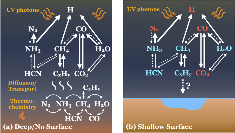
Figure 1: Diagrams describing the main chemical pathways within the atmosphere of K2-18b for a deep surface or no surface (left) and a shallow surface (right). Arrow thickness indicates the importance of each pathway, with dashed arrows being the least important. In both cases, UV photons impacting the upper atmosphere cause photochemical reactions that break down sensitive molecules such as NH3, HCN, H2O, and CH4. In the deep/no surface model, thermochemistry in the deep, hot atmosphere recreates the molecules lost to photochemistry. In the shallow surface case, atmospheric temperatures are never hot enough for thermochemistry to be effective, causing a decrease in abundances of the species in blue compared to the no surface case, and an increase for the red species. [Yu et al. 2021]

Much like within the solar system, if K2-18b has a shallow surface, the atmosphere is never hot enough for thermochemical reactions to take place, meaning the abundances of photochemically fragile species such as ammonia decrease compared to when the surface is much deeper or non-existent, as shown in Figure 1. For each version of the model, the changes in the volume mixing ratios of key chemical species within the observable atmosphere demonstrate the impacts of surfaces at different pressure levels.

four plots showing volume mixing ratios under four different surface conditions

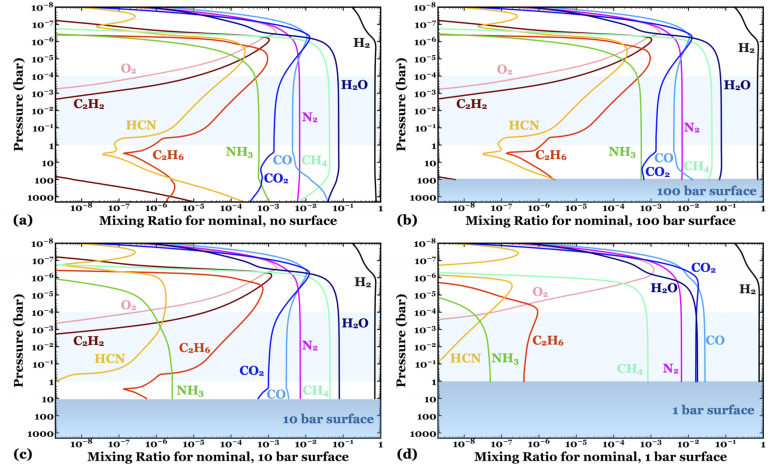
Figure 2: Plots showing how the volume mixing ratios of key chemical species change with pressure through the atmosphere of K2-18b with different surfaces. Higher pressures indicate deeper into the atmosphere. The pale blue shaded region indicates the observable part of the atmosphere. [Yu et al. 2021]

When the planet has no surface or a very deep surface, large amounts of hydrocarbons and nitrites such as hydrogen cyanide (HCN) are produced, while significant quantities of ammonia are found deep in the atmosphere just like in the case of Jupiter. When a surface exists at 10 bars, key nitrogen species can no longer be replenished and produced as easily, leading to decreasing volume mixing ratios for HCN and NH3. For the shallowest, Earth-like surfaces, thermochemistry is prevented for the majority of species, and the atmosphere is now also depleted in water (H2O) and methane (CH4). As Figure 2 shows, changing the presence or depth of a planet’s surface will change the abundances of a whole host of species — but are these changes significant enough to distinguish between surfaces?

A New Tool For Observers?

Using the finding that a variety of species are uniquely sensitive to the presence of different surfaces, the authors are able to use the abundance ratios between a species when a surface is and isn’t present, and between different pairs of species to tentatively outline a way to distinguish where a surface could be.

flowchart diagramming possibilities to identify the pressure depth of the planet surface from species abundance ratios

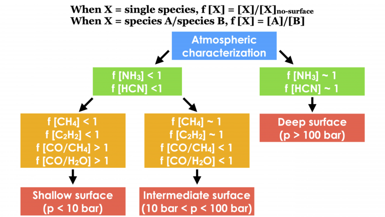
Figure 3: Flowchart to aid in the possible determination of the pressure level of a surface within an exoplanet similar to K2-18b using the observed abundance ([X]) ratios of different species. [Adapted from Yu et al. 2021]

With the flowchart shown in Figure 3 at hand, it could be possible to determine where surfaces lie within exoplanets, provided accurate abundance measurements are available. Unfortunately, current measurements of K2-18b’s Neptunian atmosphere aren’t precise enough to make a prediction about any potential surface, but upcoming JWST observations of this planet could provide further information.

So, does this mean the mystery of intermediate planet surfaces can finally be resolved? Not completely. More modelling is needed to extend the range of planetary parameters and scenarios. In the future, the flowchart could be expanded to include exciting but less well-studied species such as phosphine (PH3). The current study also does not consider the potential impacts of processes that occur on the surface, such as volcanic activity and reactions with oceans or rocks, or the potential escape of gases from the top of the atmosphere — all processes that could change the observed abundance ratios in an exoplanet. Nevertheless, today’s paper outlines an exciting new concept that extends our toolkit as we continue to try to understand the growing number of strange new worlds waiting to be explored.

Original astrobite edited by Alice Curtin.

About the author, Lili Alderson:

Lili Alderson is a first year PhD student at the University of Bristol studying exoplanet atmospheres with space-based telescopes. She spent her undergrad at the University of Southampton with a year in research at the Center for Astrophysics | Harvard-Smithsonian. When not thinking about exoplanets, Lili enjoys ballet, film, and baking.

VISTA view of the newly discovered globular cluster VVV CL001

Editor’s note: Astrobites is a graduate-student-run organization that digests astrophysical literature for undergraduate students. As part of the partnership between the AAS and astrobites, we occasionally repost astrobites content here at AAS Nova. We hope you enjoy this post from astrobites; the original can be viewed at astrobites.org.

Title: VVV CL001: Likely the Most Metal-Poor Surviving Globular Cluster in the Inner Galaxy
Authors: José G. Fernández-Trincado et al.
First Author’s Institution: University of Atacama, Chile
Status: Published in ApJL

Globular clusters are dense, spherical collections of hundreds of thousands of stars. They’re some of the oldest and most metal-poor parts of the galaxy. As such, they provide clues to the Milky Way’s past, including the galaxy merger events that may create them. Today’s paper examines the globular cluster VVV CL001 to determine its metal content and possible origins. We’ll look at how the cluster compares to others like it to see if it makes the most metal-poor podium in the Globular Cluster Olympics.

Determining the Athletes

VVV CL001 was discovered by the Vista Variables in the Via Lactea (VVV) Survey, which has increased the number of known globular clusters in the Milky Way to over 300. Think of this like the Olympic trials — this globular cluster and many others were undiscovered until they jumped out and caught the VVV Survey’s eye.

Selecting who makes an Olympic team is a difficult process, and determining which stars belong to a cluster is no different. Today’s authors used the Apache Point Observatory Galactic Evolution Experiment (APOGEE-2) and archival data to obtain spectra for stars near VVV CL001. There are a lot of stars in the field of view (or athletes in the running), so the authors had to separate out members and non-members of the globular cluster using radial velocities. Figure 1, below, shows the radial velocities in the field of view with distance from the estimated center of VVV CL001. The center of the cluster is based on proper motions from the Gaia mission. Gray points show APOGEE-2 targets, mostly near zero. Zooming into the bottom of the figure, the blue points show probable VVV CL001 stars from past studies. Those are like the athletes who have been to the Olympics before — they’re likely to qualify again. The distinct, negative radial velocities compared to other stars in the sample allowed the authors to identify two stars within the APOGEE-2 data that are also very likely members of the cluster. Those are shown in black squares.

Plot of radial velocity vs. distance from VVV CL001.

Figure 1: Radial velocities with distance to the center of VVV CL001. Stars within the cluster have a much lower radial velocity than those outside of it, making them easy to distinguish. [Fernández-Trincado et al. 2021]

Start the Match

The authors of today’s paper use a Markov Chain Monte Carlo (MCMC) method to determine the most likely age and distance of VVV CL001 based on the colors of its member stars. It turns out to be 11.9 Gyr old and 8.22 kpc from the Sun. That makes it an old, inner-galaxy cluster. And although age might not be the best criteria for judging Olympic athletes, old globular clusters are helpful because they let astronomers look back in time at what conditions were like in the galaxy in the past.

The main event in these Olympic Games is determining metal content. In this competition, the most metal-poor globular cluster is going to take home the actual medal. That’s because metal-poor clusters are usually really old and can show us what the very first generations of stars look like. Using model spectra, today’s authors fit the APOGEE-2 data for temperature, gravity, and metal content in the two VVV CL001 stars. Then they calculated the ratios of metal absorption lines in each star, like nitrogen to iron, [N/Fe], and iron to hydrogen, [Fe/H], which is used as the overall value for metal content in a star, or the metallicity.

Present the Me(t)dals

Within the orbit of the Sun, globular clusters have metallicities ranging from –2.37 to 0. Previous studies found ESO280-SC06 to be the most metal poor globular cluster in the entire galaxy, with [Fe/H] = –2.48, so that cluster is the reigning gold medalist. But VVV CL001 might give ESO280-SC06 some good competition this time around! Today’s authors found that the two stars in VVV CL001 have an average [Fe/H] = –2.45 ± 0.24. Based on the large error, it’s still unclear whether VVV CL001 has beaten ESO280-SC06 for the gold medal, but it’s certainly on the podium.

Figure 2 shows a comparison of metal ratios in the two VVV CL001 members (in black) compared to other metal-poor globular clusters (other athletes in various colors). It’s a pretty close race. In general, the clusters are similar, but VVV CL001 has a lower overall metallicity. Also, the big difference in values of [N/Fe] between the two stars in black might suggest that there are multiple populations of stars in VVV CL001, meaning that there have been multiple epochs of star formation within the cluster. It’s like VVV CL001 has some really solid older players, but the team might also include some great new up-and-comers. However, because there are only two data points, this is far from a certain conclusion.

plot showing metal abundances for various globular clusters

Figure 2: Metal abundances in metal-poor globular clusters. There is a slight horizontal offset between points for clarity. VVV CL001 has a low [Fe/H], even compared to other metal-poor clusters. [Fernández-Trincado et al. 2021]

Closing Ceremonies

The authors of today’s paper also simulated possible orbits for VVV CL001, finding that it may have been created from the Sequoia or Gaia–Enceladus–Sausage dwarf galaxies that played a big role in forming the Milky Way halo. They also found that the cluster is twice as massive as previously thought, which makes VVV CL001 one of the most massive, metal-poor globular clusters in the galaxy, and an excellent example of the extreme properties possible in a cluster. As an athlete in the Globular Cluster Olympics, it may not be the clear champion, but it is certainly unique.

Understanding globular clusters and how they are formed will provide clues that track the history of galaxies. As more and more of the clusters are identified and studied in depth by studies like the VVV Survey and APOGEE-2, we will learn more about the Milky Way and may be able to finally award the medals in the Globular Cluster Olympics!

Original astrobite edited by Sumeet Kulkarni.

About the author, Ashley Piccone:

I am a third year PhD student at the University of Wyoming, where I use polarimetry and spectroscopy to study the magnetic field and dust around bowshock nebulae. I love science communication and finding new ways to introduce people to astronomy and physics. In addition to stargazing at the clear Wyoming skies, I also enjoy backpacking, hiking, running and skiing.

Image of a field containing hundreds of visible galaxies of different colors, shapes, and sizes.

Editor’s note: Astrobites is a graduate-student-run organization that digests astrophysical literature for undergraduate students. As part of the partnership between the AAS and astrobites, we occasionally repost astrobites content here at AAS Nova. We hope you enjoy this post from astrobites; the original can be viewed at astrobites.org.

Title: New Determinations of the UV Luminosity Functions from z ~ 9 to z ~ 2 Show a Remarkable Consistency with Halo Growth and a Constant Star Formation Efficiency
Authors: R.J. Bouwens, P.A. Oesch, M. Stefanon, et al.
First Author’s Institution: Leiden University, The Netherlands
Status: Published in AJ

For decades, astronomers have used methods of “extragalactic census” to anchor our theoretical understanding of galaxy evolution. The idea is to simply measure the number of galaxies within a volume of the universe as a function of some physical variable (like dark matter halo mass, stellar mass, or luminosity, for instance). When measured at one epoch or point in time, these censuses tell us a great deal about the universe by simply recording how common galaxies of different types are. If this measurement is carried out at various redshifts (z), one obtains a timeline of the universe that encodes the changes in the underlying galaxy population according to the variable in question.

Photograph of a space telescope above the earth.

Photograph of the Hubble Space Telescope. [NASA]

Consider the ultraviolet (UV) luminosities of galaxies. The number of galaxies in a given volume as a function of UV luminosity has the catchy name of the UV luminosity function. The UV luminosity function is a particularly useful probe in galaxy evolution studies, since the UV luminosity of a galaxy is strongly correlated with its star formation rate (newly formed stars are bright in the UV). This means that if we can measure the evolution of the UV luminosity function across the history of the universe, we can investigate the growth of stars within galaxies across cosmic time. Since this extragalactic census is purely observational, it is completely agnostic about the underlying physics of star formation. However, these types of measurements are nonetheless invaluable for theorists. Census-like observations like the UV luminosity function provide bedrock constraints for theories of galaxy evolution, because at the end of the day, any working model of galaxy evolution must be capable of reproducing them. The goal then is to obtain the most precise censuses possible.

In today’s astrobite, we explore a recent effort to obtain the premier measurements of the evolution of the UV luminosity function using observations from the Hubble Space Telescope.

Tackling the UV Luminosity Function with Hubble

This work combines nearly all of the deepest survey observations conducted with the Hubble Space Telescope (HST) to obtain the largest selection of galaxies at z > 2 to date from this facility. Their primary sample contains some 24,000 galaxies, making it more than twice as large as previous selections of galaxies from HST surveys. To measure the evolution of the UV luminosity function, galaxies are first grouped into redshift slices of width 1 in redshift space, from z ~ 2 to z ~ 9 (for example, galaxies within 1.5 < z < 2.5 are grouped together at z ~ 2). To achieve this, the team first uses the well-tested “drop-out” method (see this astrobite for another detailed explanation). A strong spectral feature in star-forming galaxies is the Lyman break at 912 Angstroms, where flux at shorter wavelengths is absorbed by gas in the intergalactic medium. At a given redshift, it is possible to fairly accurately exclude low-z galaxies by selecting only sources with significant flux at wavelengths longer than the Lyman break (their flux “drops out” at shorter wavelengths). For an even cleaner sample, the team also models the spectral energy distributions of the galaxies in their sample, comparing their observed photometry to model galaxy templates. This yields a distribution of possible redshifts for each source and an associated probability, which is used to exclude the color-selected galaxies that may in fact be low-z interlopers.

With the approximate redshift of each galaxy known, it is possible to infer its absolute magnitude and finally measure the UV luminosity function. Before measuring the UV luminosity function, they add to their dataset the constraints from several other efforts, including ground-based observations and a recently selected sample of galaxies at z ~ 10 from another work. The final UV luminosity functions at each redshift slice is shown below in Figure 1, tracking its evolution from z ~ 10, when the universe was 0.48 billion years old, to z ~ 2, when the universe was 3.3 billion years old.

plot of the number of galaxies in a given volume vs. the UV luminosity

Figure 1: The UV luminosity function measured in this paper at each redshift between 2 < z < 9, plus that measured at z ~ 10 in another work (Oesch et al. 2018). Across this ~ 3 billion year time period, the number density of all galaxies increases by orders of magnitude, with fainter galaxies becoming less dominant over time. [Bouwens et al. 2021]

Extracting Extragalactic Information

As can be seen from Figure 1, interpreting the changes in the UV luminosity function between 2 < z < 10 is complicated. To simplify the matter, the authors model the UV luminosity function at each redshift with a parameterization known as a “Schechter function.” This model combines a power law at the faint end and an exponential decline on the bright end. It has three free parameters: α, the slope of the faint-end power law; M*, the absolute magnitude where the slope changes from power-law behavior to exponential; and φ, the normalization. The Schechter function fits to the data are also shown in Figure 1.

three plots showing the evolution with redshift of the three schechter function parameters.

Figure 2: The evolution of the Schechter function parameters as measured in this work. The remarkable result presented in this paper is demonstrated in the top panel: The evolution of alpha in the UV luminosity function almost matches perfectly with the evolution of the low-mass end of the dark matter halo mass function, supporting a fundamental link between dark matter halo mass and star formation in galaxies. [Bouwens et al. 2021]

The evolution of each of the Schechter parameters in the UV luminosity function tells us something physical about star formation in galaxies throughout cosmic time. The measured trends in these parameters are shown in Figure 2. As can be seen, the faint-end slope (α) follows a strongly linear relationship with z and becomes a weaker power law over time, indicating that brighter galaxies become more common from early times to later times. The turnover magnitude (M*) stays roughly constant until a dramatic change at z ~ 2.5, where it is thought that the most massive and bright galaxies begin to quench and fade in the UV. Finally, the normalization (φ) smoothly increases across cosmic time and flattens out near z = 0, indicating a smooth growth in the overall number density of galaxies.

What is most interesting, the authors note, is that the faint-end slope evolution almost identically matches the evolution of the dark-matter (DM) halo mass function (the number of galaxies per unit volume as a function of DM halo mass). In fact, if one assumes a constant efficiency of turning gas into stars within a given DM halo, and applies this assumption to the dark-matter halo mass function, the trends shown in Figure 1 are almost exactly reproduced. This supports an intimate link between the DM halo mass of galaxies and their ability to form stars.

By combining all of the existing survey fields observed by HST, the authors obtained a precise characterization of the UV luminosity function across a dramatic three billion years of our universe’s history, from 2 < z < 10. With the imminent launches of the Roman Space Telescope (and its enormous field of view, 100x that of HST!) and the James Webb Space Telescope (with its extreme infrared sensitivity), we can be confident that our understanding of the universe will only grow from here.

Original astrobite edited by Alex Pizzuto.

About the author, Lukas Zalesky:

I am a PhD student at University of Hawaii’s Institute for Astronomy. I am interested in understanding the way galaxies form and evolve over billions of years, as well as gravitational lensing by galaxy clusters. Outside of research I spend my time with animals, exercising, practicing Zen, and exploring the beautiful island of Oahu.

Two images — one wide-field and one zoomed in — show a small, compact dwarf galaxy.

Editor’s note: Astrobites is a graduate-student-run organization that digests astrophysical literature for undergraduate students. As part of the partnership between the AAS and astrobites, we occasionally repost astrobites content here at AAS Nova. We hope you enjoy this post from astrobites; the original can be viewed at astrobites.org.

Title: A recently quenched isolated dwarf galaxy outside of the Local Group environment
Authors: Ava Polzin, Pieter van Dokkum, Shany Danieli, Johnny P. Greco and Aaron J. Romanowsky
First Author’s Institution: Yale University
Status: Accepted to ApJL

Earth Orbit — Hubble

A mock-up of a daily newspaper front page named "Astrobites News". The headline of the article is "Teenage Galaxy Eludes Authorities" and an image of a galaxy is captioned "COSMOS-dw1 eluded authorities for far too long." A teen galaxy, going by the name COSMOS-dw1, refuses to testify to authorities (i.e., scientists) about its nature or, for that matter, about anything much at all.

The young specimen has been taken into custody (i.e., was discovered) recently and created more questions than it answered. Specifically, it appears to have quenched all star formation processes, feeding once again into unfounded prejudice about young “slacker” galaxies. Why it has done so, it refuses to imply directly. One would naturally assume that such staggering behavior must be a direct consequence of the environment of such a young, impressionable galaxy. But authorities were stunned when they learned that COSMOS-dw1 exists in isolation, acting as a lone wolf. An attempt to identify possible accomplices is underway, however none make convincing suspects thus far. Further investigation will be necessary to persuade the galaxy to cooperate and for us to learn more about this puzzling behavior.

An Addition to the Collection

Alright, this fictional newspaper snippet may simplify things a little. But it does provide a nice overview on the newly discovered young dwarf galaxy COSMOS-dw1, a (most likely) quenched galaxy outside of the Local Group, found by a stroke of luck. A galaxy is considered quenched if it has shut down all star formation. These small galaxies are fairly underrepresented in contemporary surveys, due to the bias of larger galaxies with high surface brightnesses being much easier to find.

In the context of galaxies, “small” or “low mass” refers to galaxies with masses below 10solar masses (the Milky Way has roughly 1012 solar masses). The galaxy discussed in today’s paper is named COSMOS-dw1 and was discovered in archival Hubble Space Telescope data in the so-called COSMOS-CANDLES field, one of the most observed regions of the sky. It showed up as a semi-resolved object within the data, which suggests that it cannot be too far away.

But COSMOS-dw1 is not only interesting because it adds to our short list of well-documented low-mass galaxies, but also due to a number of further notable features: it displays a rather asymmetric shape with a clump of blue stars (which are hotter, heavier, and much more short-lived than yellow or red stars) off-center to the north (see Figure 1). The rest of the stellar population appears to be much older — most likely post-main sequence — and is distributed more evenly.

Two-panel figure shows a color-magnitude diagram on left, with some data points in blue, and an image of a small, dense galaxy on the right.

Figure 1: Color–magnitude diagram of COSMOS-dw1 (left). The blue points refer to the bright blue stars marked in the RGB image of the galaxy (right). [Adapted from Polzin et al. 2021]

Missing Lines

In order to learn more about the galaxy, spectroscopic observations were taken by the authors with the Low Resolution Imaging Spectrograph (LRIS) on the Keck I telescope in Hawaii. A distance of around 22 Mpc was deduced from the measurements, and the galaxy’s radius was determined to be around 450 pc (around 127 times smaller than the Milky Way), with a mass of 2.4 x 10⁶ solar masses.

Arguably the most important information obtained from the spectroscopy measurements is the absence of emission lines, specifically H-alpha emission lines. In galaxy research, the brightness of the H-alpha line indicates the number of massive stars within that galaxy, which can be used to infer the rate of star formation. Massive stars ionize the gas around them. The hydrogen recombination produces line emission, such as the well-known Balmer-series lines of H-alpha and H-beta. The lack of H alpha emission suggests that the galaxy is in fact quenched, i.e., it does not produce any new stars at the moment. However, strong Balmer absorption is visible, implying the presence of A-type stars at an age of roughly 1 Gyr. Figure 2 displays the spectrum of COSMOS-dw1 and the location of where H-alpha emission would be expected, as a function of wavelength.

Spectrum for COSMOS-dw1, showing several spectral lines but no evidence of H-alpha.

Figure 2: LRIS spectrum of COSMOS-dw1 in black with the best-fit model overplotted in pink. The gray area on the right shows the wavelength range where H-alpha emission would be expected. [Adapted from Polzin et al. 2021]

From the color–magnitude diagram (seen in Figure 1) it is evident that within COSMOS-dw1, a population of bright, very blue stars exists within a rather complex stellar population. The location of these stars provides an upper limit for the age of the galaxy. As stars age, they disperse throughout their host galaxy. Since these blue stars are quite close to the center, it can be inferred that the galaxy is young.

A Lone Wolf

So, why has this young galaxy ceased all star formation, at least for the moment? The authors point out that usually dwarf galaxies are quenched due to environmental effects, such as ram pressure — the process of pressure from the environment stripping a small galaxy of the gas essential for star formation as the galaxy falls towards a larger mass.

For any kind of environmentally caused quenching, one would expect to see a bright companion galaxy close to the dwarf galaxy. Intriguingly, such a companion is nowhere to be found for COSMOS-dw1. The authors have searched the immediate surroundings of the dwarf galaxy and found only two galaxies that exceed the minimum mass to be considered a “luminous neighbor”. However, it appears these are too far away to be responsible for the quenching. Additionally, the complex stellar population within COSMOS-dw1 suggests that star formation started and stopped several times in the past. We also know that the quenching happened rather recently due to the population of rather young stars.

Supernovae to the Rescue!

The authors propose a different mechanism responsible for quenching: internal feedback from supernovae. This basically means that a violent process such as a supernova may inject energy and momentum into the interstellar medium — enough maybe to shut off star formation, at least temporarily. The clump of blue stars found within COSMOS-dw1 may be the location of this feedback event.

More surveys may help us to better understand these dwarf galaxies. The authors note that finding this quenched small galaxy in such a well-studied field in the sky suggests that they are fairly common.

While we are quite calmly and comfortably existing in a side arm of a spiral galaxy that does not currently experience any violence, it is exceedingly interesting to take a look at other galaxies, especially outside the Local Group, to gain a perspective on the many altering processes happening to other galaxies and the star formation within. Space is always dynamic; even if an object such as COSMOS-dw1 exists in isolation, rapid exchange of energy and great change can always come from within.

Original astrobite edited by Alex Pizzuto.

About the author, Jana Steuer:

I’m a second year PhD student at the LMU Munich, working for the University Observatory (USM), which owns the 2.1m Fraunhofer Telescope Wendelstein. My field of research is exoplanets. I hunt for traces of them in data from big surveys, like the TESS mission and then follow them up, using spectroscopy and photometry. Mainly, I focus on long period planets that may potentially harbor life. When I’m not planet hunting, I act as a DM for several Dungeons and Dragons groups and annoy people with facts from Tolkien’s Silmarillion. I enjoy kickboxing and learning about ancient human history.

Simulation still showing the formation of the cosmic web

Editor’s note: Astrobites is a graduate-student-run organization that digests astrophysical literature for undergraduate students. As part of the partnership between the AAS and astrobites, we occasionally repost astrobites content here at AAS Nova. We hope you enjoy this post from astrobites; the original can be viewed at astrobites.org.

Title: Cosmic Velocity Field Reconstruction Using AI
Authors: Ziyong Wu et al.
First Author’s Institution: Sun Yat-Sen University, China
Status: Published in ApJ

Going with the (Hubble) Flow?

Hubble’s law is a beautifully simple statement: a galaxy caught in the Hubble flow, moving with the expansion of the universe, should be traveling away from us at a speed proportional to its distance. Unfortunately, however, this velocity–distance relation is too good to be true: due to the pesky influence of gravity, Hubble’s law is invalid in the vast majority of cases. In general, a galaxy’s net motion can be attributed to a combination of the Hubble flow, the galaxy’s motion within its galaxy cluster or group, and the motion of the cluster or group itself. We collectively refer to these deviations from the Hubble flow as “peculiar motions” or “peculiar velocities.”

While the presence of peculiar motions spoils the simplicity of Hubble’s law, these motions can be a blessing in disguise: since diversions from the Hubble flow are caused by gravitational interactions — and therefore by the presence of matter —  peculiar motions serve as excellent probes for the physics of structure in the universe. Peculiar velocities have been used to map the cosmic web — the vast network of filaments connecting matter on the universe’s largest scales (explored further here, here, and here) — and are linked to the dynamics of galaxy clusters and the cosmic microwave background via the kinematic Sunyaev–Zel’dovich effect. Peculiar motions are also the root cause of redshift–space distortions, and thus one requires precision measurements of peculiar velocities in order to test cosmological models using the Alcock–Paczynski effect (see here and here for deeper explanations of this technique).

One caveat, though: measuring peculiar velocities is hard. To decouple peculiar motions from the Hubble flow observationally, we need a means of measuring distances that doesn’t require redshifts. To this end, a distance ladder or the Tully–Fisher and Faber–Jackson relations are viable methods, but each carry significant measurement uncertainty. Alternatively, we can take a theoretical approach, using perturbation theory to infer cosmic velocities from cosmic density data. However, any attempts to fully model the nonlinear growth of large-scale structure by hand quickly become prohibitively complex, necessitating a number of approximations and simplifications. How, then, can we accurately and efficiently compute peculiar velocities on cosmological scales? The authors of today’s paper may have found a solution in the field of machine learning: convolutional neural networks.

From Convolutions to Cosmology

Artificial neural networks are, in essence, models with very many free parameters. As one trains the neural network by feeding it many input data sets and scoring its output against the expected results, the network adjusts its parameters, thus learning how best to map the given inputs to the desired outputs. Figure 1 shows a simple neural net with a fully connected three-layer “feed-forward” architecture; the data, in the form of an array of real numbers, is reprocessed as it’s transmitted from the “input layer” to a “hidden layer” and finally to the “output” layer. Each connection between layers bears a weight that dictates how a layer’s “neurons” should process their inputs — these weights are the free parameters in the neural network. Ultimately, neural nets produce models that are highly nonlinear, thus making them ideal for studying the complex dynamics of cosmic structure formation.

Diagram of an interconnected group of nodes

Figure 1: A schematic diagram of a fully connected three-layer feed-forward neural network, where each circle represents a neuron. Here, the data is fed into the input layer as an array, then transmitted to the hidden layer where it is mixed and reprocessed based on the weights of the connections leading into the hidden layer; the resulting values are sent to the output layer, where they are reprocessed one final time, ultimately producing a highly nonlinear model. [Glosser.ca]

Typically, neural networks contain many hidden layers, and thus possess an obscene number of parameters — in this paper, the authors use a network with 48,690,307 parameters! With this many parameters, neural nets run the risk of overfitting the data, using up a large amount of memory, and running extremely slowly. Fortunately, one can ameliorate these issues by adding one or more “convolution” layers to a network, filtering and contracting the data and preserving only the most salient features (for a more thorough explanation of this convolution process, see here); this is especially useful when processing detailed image data, such as the cosmic density maps that the authors use as their input data. The authors optimize their network by adopting a U-Net architecture, which employs a series of convolutions followed by a series of deconvolutions to quickly parse the input and highlight its key components.

To generate their training and testing data sets, the authors simulate the formation of large-scale structure up to the present day, retrieving both cosmic density and momentum maps; the density maps are used as inputs to the neural net, while the corresponding velocity maps — computed by dividing the momentum fields by the density fields — are used to evaluate the neural net’s output and to subsequently train, cross-validate, and test the resulting model.

Math vs. Machine

The authors assess the performance of their trained neural network by comparing its peculiar velocity predictions to those of linear perturbation theory. In nearly all cases, the neural net clearly outperforms the theoretical model. Perturbation theory performs well in regions of low density and velocity, occasionally yielding better predictions than the neural net. However, in regions of high density and velocity and in merger situations where two regions of opposing velocity collide with one another, perturbation theory fails completely, while the neural net still faithfully reconstructs the velocity field (see Figure 2). Over multiple testing data sets, the neural net is shown to be robust in all situations, while perturbation theory becomes practically useless in the presence of nonlinear dynamics.

six panel plot evaluating the neural net results

Figure 2: Comparison of a simulated velocity field (upper left) with a field predicted by the neural network (upper middle) and by perturbation theory (upper right); the lower left shows the underlying density field, while the lower middle and lower right show the residuals for the neural net predictions and the perturbation theory predictions, respectively. In regions of high density and velocity and in regions of converging flow, perturbation theory breaks down. [Wu et al. 2021]

While the neural network used in this paper can definitely be improved — perhaps by further optimizing its architecture or by using more training data — the authors have shown that neural nets can be valuable tools for predicting peculiar velocities. With such programs as DESI, EUCLID, the Rubin Observatory, and the Nancy Grace Roman Space Telescope promising to map out an unprecedented volume of the cosmos within the next decade, it is of utmost importance that we possess fast and accurate methods for parsing the new data — and neural networks are surely at the forefront of these methods. Maybe the rise of machines isn’t such a bad thing after all!

Original astrobite edited by Pratik Gandhi.

About the author, Ryan Golant:

I am a first-year astronomy Ph.D. student at Columbia University. My current research involves the use of particle-in-cell (PIC) simulations to study magnetic field growth in gamma-ray burst afterglows and closely related plasmas. I completed my undergraduate at Princeton University, and am originally from Northern Virginia. Outside of astronomy, I enjoy playing violin, studying art history, reading Wikipedia, and watching cat videos.

Spitzer photograph of a dramatic nebula surrounding bright point sources.

Editor’s note: Astrobites is a graduate-student-run organization that digests astrophysical literature for undergraduate students. As part of the partnership between the AAS and astrobites, we occasionally repost astrobites content here at AAS Nova. We hope you enjoy this post from astrobites; the original can be viewed at astrobites.org.

Title: The consistency of chemical clocks among coeval stars
Authors: Francisca Espinoza-Rojas et al.
First Author’s Institution: Pontifical Catholic University of Chile
Status: Submitted to ApJ

Stellar age is an extremely valuable parameter to constrain because it introduces time into our study of astronomical objects. Pairing the observed properties of stars with time opens up a rich new dimension in the study of our galaxy and beyond. For example, when we pair stellar age with stellar kinematics, we can dynamically trace stars back to their birth locations to study things like galactic evolution and star formation in detail. When we consider stellar age in our study of exoplanets, we can peer into the planet formation and evolution process. When we pair stellar age with stellar chemical abundances, we can trace the evolution of specific elements over time in the galaxy. Weaving time into these various analyses opens up a new realm of insight that enhances our understanding of the universe. However, with this all said, stellar age is extremely difficult to constrain.

Stellar Ages Are Hard to Determine

Some methods of constraining stellar ages include using photometry, dynamics, gyrochronology, and the abundances of individual elements like lithium in stars. For example, the locations of stars on the color–magnitude diagram (CMD), which are determined by photometry, can hint at stellar age. Many stellar and galactic astronomers fit isochrones, lines of constant age in the CMD, to the photometric data of a single or group of stars to estimate their age. However, this method relies on very well-constrained dust parameters between the observer and the object. Gyrochronology, using stellar rotation to estimate age, is another effective method, but it requires knowledge of the inclination of the star, something that is often difficult to determine. We can also use lithium abundances to estimate stellar age. Lithium, however, is only an effective age indicator in young stars with convective envelopes. As you can probably tell, there are tons of ways to estimate stellar age, but they all suffer from various limitations and uncertainties.

Abundance Ratios of Certain Elements Track with Age

An interesting, and somewhat new, avenue for probing stellar age is through the use of chemical clocks. Chemical clocks are sets of elemental abundance ratios that have been observed to track with stellar age. The idea behind chemical clocks is rooted in the notion that different families of elements are expelled into the interstellar medium (ISM) on different time scales (see Figure 1). For example, elements like Mg, Al, and Ti are produced in dying massive stars, which live short lives that end in core-collapse supernovae. As a result, these elements follow very different timescales than, say, Ba and Y — elements that are produced primarily in low-mass stars, which have much longer lifetimes and subsequently take longer to spread their nucleosynthetic products out into the ISM. This means that the ratios of various abundances in the ISM are constantly changing. When a star is born, it traps with it the chemical abundances of the ISM at the time of its birth like a time capsule and carries them with it throughout most of its life. Thus, the ratios of certain elements in a star could probe at what point in the Milky Way’s chemical evolution (and thus in time) the star was born.

diagram showing sources of chemical enrichment over time

Figure 1: A cartoon depicting the different timescales of chemical enrichment from various sources, the concept behind chemical clocks. Core-collapse supernovae, which come from short-lived massive stars, for example, dominate the chemical enrichment of the Milky Way early on. Asymptotic Giant Branch (AGB) stars, which originate from long-lived low- and intermediate-mass stars, start contributing to galactic chemical enrichment later on. [Jacobson & Frebel 2014]

Testing Chemical Clocks in Wide Binaries

The authors of today’s paper set out to investigate just how reliable chemical clocks are at keeping time by testing their consistency in wide binaries. Wide binaries are pairs of stars that were born together and orbit a common center of gravity. As their name implies, wide binaries have large separations, making them easier to study observationally. These systems are a great way to test chemical clocks because they consist of two stars that share an age. Today’s authors investigate various chemical clock abundance ratios in 36 pairs of wide binaries to see which chemical clocks are most consistent among stars born at the same time.

The authors are first able to recreate the result found in previous studies that wide binaries are more chemically similar in their elemental makeup than random pairs of stars in the field. This makes sense. Stars born in the same place should share the same chemical composition because the interstellar medium is understood to be very homogeneous on small spatial scales. The chemical abundances of stars directly reflect the chemical abundances of the material from which they were born, so if the interstellar medium is well-mixed, and stars share a birth place and age, then they should share a similar chemical profile.

42-panel plot exploring different abundance ratios among the binary pairs

Figure 2: The consistency in the abundance of various chemical clocks between both components of wide binaries. The x-axis in each subplot is the abundance in the indicated chemical clock for one component of the binary (A), and the y-axis is the same for the other component (B). The tighter the 1-to-1 relationship in a subpanel, the more consistent a chemical clock between stars in the binary pair. [Sc/Ba], [Al/Ba], and [Ti/Ba] (all in the 4th row), among others, stand out as chemical clocks that appear to be promising age indicators. [Espinoza-Rojas et al. 2021]

The authors then make an interesting discovery: when they investigate chemical clocks among wide binaries, they find that components of wide binaries tend to be even more similar in chemical clock abundances than other elemental abundances, as seen in Figure 2. They find that even when components of a wide binary are quite dissimilar chemically in [X/Fe], as is the case in one particular pair in their sample (black box in Figure 2), they are still very consistent in chemical clock abundances. This result suggests that chemical clocks could be effective age indicators even when stars are extremely dissimilar in other elements. The authors highlight that three chemical clocks in particular, [Sc/Ba], [Al/Ba], and [Ti/Ba], seem to be the most consistent among wide binaries and thus the most promising indicators of age.

What is next for the field of chemical clocks? One new avenue involves calibrating chemical clocks using stars with ages derived through other means, such as gyrochronology. This way, we can create an empirical, observed relationship between a star’s abundance in a chemical clock and its age. These empirical relationships will likely vary with Milky Way location, but they will open up a new avenue of probing stellar age in stars with a variety of parameters. With chemical clocks, we can hopefully expand our stellar age toolbox and allow for more checks on stellar age, an important parameter in observational astronomy.

Original astrobite edited by Lili Alderson.

About the author, Catherine Manea:

Catherine is a 2nd year PhD student at the University of Texas at Austin. Her research is in galactic archaeology, the practice of using the kinematic and chemical information of individual stars to study the evolution of our Milky Way. She is particularly interested in pushing chemical tagging, the practice of tracing stars back to their birth sites, to new limits.

Photograph of a galaxy undergoing ram pressure stripping

Editor’s note: Astrobites is a graduate-student-run organization that digests astrophysical literature for undergraduate students. As part of the partnership between the AAS and astrobites, we occasionally repost astrobites content here at AAS Nova. We hope you enjoy this post from astrobites; the original can be viewed at astrobites.org.

Title: ELVES I: Structures of Dwarf Satellites of MW-like Galaxies; Morphology, Scaling Relations, and Intrinsic Shapes
Authors: Scott G. Carlsten et al.
First Author’s Institution: Princeton University
Status: Accepted to ApJ

Dwarf galaxies are thought to be incredibly suggestible; there has been a range of diverse dwarf galaxies observed in our universe, indicating that they are extremely sensitive to their surroundings. The observed differences in sizes, shapes, and colours of dwarf galaxies is believed to be at least in part due to differences in the environment they inhabit. All galaxies are thought to be surrounded by a halo of dark matter (see this astrobite for more details). Many dwarf galaxies are satellite galaxies, meaning that they are found in orbit within a larger host dark matter halo that also typically contains a larger central galaxy (for example, the Small and Large Magellanic Clouds are satellite galaxies, both in orbit of our own Milky Way).

Satellite galaxies are subject to many different interactions with their host dark matter halo. These interactions between a satellite galaxy and its host can have devastating effects on the satellite galaxy itself. For example, their gas content can become extremely disturbed (and sometimes completely removed) by ram pressure stripping, which can eventually bring star formation in the satellite to a halt (see this astrobite for a summary of the seminal paper on ram pressure stripping). Similarly, their stars are subject to tidal stripping, which arises due to differences in the gravitational potential of the satellite galaxy and its host.

6-panel image showing photos of different types of dwarf galaxies

Figure 1: Examples of dwarfs visually classified as early-type (ETG) and late-type (LTG). Late-type dwarfs are irregular, with apparent active star formation throughout the galaxy while early-types are smooth and featureless without any star-forming clumps. [Carlsten et al. 2021]

Despite the observed diversity of dwarf galaxies, they can broadly be classified into two morphological types: late-type and early-type (see Figure 1 for examples). Late-type galaxies are typically star-forming, whereas early-type galaxies lack star-forming regions and appear smoother than late-types. Today’s paper uses the ongoing Exploration of Local VolumE Satellites (ELVES) Survey to investigate how the structural properties of dwarf galaxies can change depending on the environment and morphology of the galaxy. The galaxies in the ELVES sample are all within the Local Volume (D < 12 Mpc), and are satellite galaxies in orbit of Milky Way-like halos.

Going from a Late-type to an Early-type?

The current picture of dwarf galaxy evolution suggests that early-type dwarfs are formed from late-type dwarfs interacting with a host halo. If this is the case, then early-type dwarfs can be thought of as dwarf galaxies in the last throes of their evolution, and any differences in characteristics of late-type and early-type galaxies could provide insights into the physical mechanisms behind this evolution (such as the removal of star-forming gas through ram pressure stripping).

Plot of effective radius vs. log stellar mass for dwarf galaxies

Figure 2: Log effective radius vs. log stellar mass for the dwarf galaxies in the Local Volume sample. The upper panel displays points for each dwarf galaxy in the sample, with red indicating early-type and blue indicating late-type. The bottom panel shows average trends binned by stellar mass. The dashed lines show the mass-size relations for early-type (red) and late-type (blue) dwarf galaxies of higher stellar mass from the GAMA Survey. [Adapted from Carlsten et al. 2021]

To investigate whether there are any structural differences between early- and late-types, the authors plot the effective radius of the dwarf galaxies in their sample (essentially the galaxy’s size) by their stellar mass. It can be seen from Figure 2 that there is no significant difference between the early- and late-type galaxies at fixed stellar mass. This similarity between late-types and early-types suggests that the physical processes relevant in forming early-type galaxies (such as ram pressure stripping) do not necessarily induce any change in the galaxy’s size. These results indicate that the transformation process from late-type to early-type requires only the removal of the galaxy’s star-forming gas — significant structural change to the galaxy is not necessarily required. Also of note is the difference between the author’s results, where the sample is limited to dwarf galaxies with M* < 108.5 M and results for satellite galaxies with higher masses (indicated by the blue and red lines in the bottom panel of Figure 2). The authors suggest that this difference hints that there is a characteristic stellar mass scale, above which additional physical processes may be required to explain the sudden difference in sizes between early- and late-types.

Environmental Effects

The next question the authors aim to answer is: how does the mass of the dwarf galaxy’s host dark matter halo affect the evolution of the dwarf galaxy? To consider this, the authors again compare the sizes of dwarf galaxies. This time, a comparison is made between dwarf galaxies that are orbiting within larger cluster environments and the dwarf galaxies in their Local Volume environment.

Plot showing mass–size relations for cluster and field dwarf galaxies

Figure 3: The mass–size relations of the cluster (grey) and field (cyan) dwarf samples normalized to the full Local Volume sample (green). At fixed stellar mass, the cluster sample is offset to larger sizes, whereas the isolated field sample is offset to smaller sizes. Field galaxies are isolated dwarf galaxies that have been taken from an auxiliary sample, using additional observational data. [Adapted from Carlsten et al. 2021]

As can be seen in Figure 3, dwarf galaxies in cluster environments tend to be slightly larger than dwarf galaxies in the Local Volume at a fixed stellar mass. The authors argue that the observed increase in size is down to more intense tidal stripping and heating of galaxies in extreme cluster environments, which aligns with theoretical expectations. While an ~8% increase in sizes for the dwarfs in cluster environments is observed, the authors note the mass–size relation is strikingly similar between the two environments, especially since the mass of the host dark matter halos differ by a factor of 10. This is perhaps indicative that the exact environment plays a fairly small role in dwarf galaxy evolution — a somewhat surprising result!

In conclusion, today’s authors are able to gain insights into the physics of dwarf galaxy transformation from late-types to early-types, and how these processes vary between the Milky Way-like and cluster environments. The authors comment that a comparison with simulations will be useful in constraining the physics of how dwarf galaxies evolve. Their observational results have quantified the start and end points of the transformation, and simulations may now be able to tie them together to tell the middle part of the story!

Original astrobite edited by Luna Zagorac.

About the author, Katy Proctor:

I am a first-year PhD student at the International Centre for Radio Astronomy Research at the University of Western Australia. My research is focused on using cosmological simulations to study the evolution of satellite galaxies. Outside of research, I can usually be found climbing up walls or playing guitar.

Photograph of a blue planet

Editor’s note: Astrobites is a graduate-student-run organization that digests astrophysical literature for undergraduate students. As part of the partnership between the AAS and astrobites, we occasionally repost astrobites content here at AAS Nova. We hope you enjoy this post from astrobites; the original can be viewed at astrobites.org.

Title: Eccentric Early Migration of Neptune
Authors: David Nesvorný
First Author’s Institution: Southwest Research Institute
Status: Published in ApJL

Among the furthest reaches of our solar system, beyond the orbits of the mighty ice giants, lies the Kuiper Belt. This circumstellar disk, roughly twenty times as wide as the asteroid belt, is home to many small bodies (defined by the IAU as any Sun-orbiting body that is neither a planet, dwarf planet, nor satellite), as well as various dwarfs, including what was once the ninth planet. Collectively, these bodies are referred to as Kuiper Belt Objects (KBOs), which are themselves a subset of Trans-Neptunian Objects (TNOs). Understanding the collective orbits of KBOs provides important insights into the evolutionary history of our early solar system.

Neptune, like other outer gas giants, is known to have migrated in the past and interacted with KBOs. We can predict what Neptune’s migratory orbit was like by simulating different planetary migration scenarios for the outer planets, seeing how they affect KBOs, then finding the parameters that best match currently observed KBO orbits. Today’s paper examines a group of KBOs within a specific range of orbital parameters whose current orbits are unable to be accounted for in simulations if Neptune migrated with a low orbital eccentricity (<< 0.03). Instead, better results are obtained if Neptune migrated with a higher eccentricity of e ~ 0.1.

Space For The Travelling Planet

Under the current framework for accounting for the dynamical evolution of the early solar system, Neptune is known to have migrated into a higher orbit, subsequently interacting with the Kuiper Belt and its various KBOs. After this migration, Neptune’s orbit slowly decayed and circularised, causing the planet to move inward to its current position today. This migration is noted to have altered the distribution of inclinations and eccentricities of KBOs, and (in conjunction with other migrations by Uranus, Saturn, and Jupiter) is theorised to be responsible for scattering many KBOs and other planetesimals into the inner solar system (the Late Heavy Bombardment). Studies focusing on this period of instability have aimed to constrain the eccentricity of Neptune’s migration. There are many factors to consider, such as tidal interactions and possible orbital resonances with KBOs or the other gas giants, dynamical friction, and Kozai cycles (which cause eccentricity and inclination to oscillate).

This study definitively rules out the low-eccentricity migration scenario, and instead provides support to an excitation scenario wherein Neptune had an eccentricity of e ~ 0.1.  The data used to fine-tune the simulations was obtained from the Outer Solar Systems Origin Survey (OSSOS), which identified a population of KBOs with semimajor axes between 50 and 60 AU, a perihelion distance greater than 35 AU, and an inclination of less than 10 degrees. Figure 1 shows all KBOs with semimajor axes between 50 and 60 AU plotted by eccentricity, with the OSSOS samples highlighted as blue triangles. Simulations show that the existence of this population is easily accounted for in the high-eccentricity model; here bodies originally at around 30 AU are scattered into higher orbits (50 to 60 AU), where they subsequently interact with Neptune due to mean motion resonances. The bodies eventually decouple, forming the specific 50–60 AU population that we see today.

Plot showing eccentricity vs. semimajor axis for KBOs

Figure 1: A plot of modelled orbits of KBOs with semimajor axes between 50 and 60 AU plotted by eccentricity (shown as red dots), with the OSSOS detections overlaid as blue triangles. [Nesvorný 2021]

A Wandering Neptune

Importantly, this study provides a key physical explanation as to why the low-eccentricity model cannot work in practice. Were Neptune to have a low eccentricity, the mean motion resonances would not be as effective, and so the scattered KBOs would need to decouple via Kozai resonances. However, in Kozai cycles, as eccentricity decreases, inclination must increase. The KBOs in this situation would thus be unable to satisfy the target parameter range of having less than 10 degree inclination (see Figure 2, which shows this exclusionary zone). The only other explanation for their existence is that these KBOs originated in situ, in some hypothetical disc that was perturbed by other means.

2-panel plot of inclination vs. perihelion distance for KBOs under 2 models.

Figure 2: Orbital inclinations and perihelia for KBOs with semimajor axes between 50 and 60 AU. Left and right panels correspond to two different dynamical models. Blue triangles denote the OSSOS samples. The olive shaded region is the excluded region in which objects scattered by a low-eccentricity Neptune cannot exist. The fact that OSSOS samples do exist rules out the low-eccentricity case. [Nesvorný 2021]

Questions remain over the exact cause of Neptune’s high-eccentricity migration in the first place. One scenario involves a mean motion resonance between Uranus and Neptune, but it is rare for such effects to alter eccentricity by the degree required (of order 0.05). Comparatively, encounters with Saturn and Jupiter do have the potential to propel Neptune into a highly eccentric orbit (of order 0.2), but such scenarios do not reconcile with KBO observations. Instead, the most likely scenario is that Neptune had an encounter with a rogue planet. Such a planet would need to have been at least as massive as the Earth, though detailed predictions of possible trajectories are, as yet, unable to be gleaned from the current KBO population nor from simulations. That said, based on the current KBO population, it is possible to estimate how many Earth-like planets could have been in the outer solar system; one study gives an 68% likelihood of fewer than 3.

And Yet They Moved

The Kuiper Belt remains an active frontier for research into the dynamical evolution of the early solar system. Not only does accounting for the orbital properties of KBOs yield insights into the evolutionary history of the outer planets, but it enhances our understanding of the physical processes at play — from mean motion resonances to Kozai cycles — allowing us to better constrain the orbital parameters of migrating planets. This is important given the rise of exoplanetary science, and the need to account for the many exotic planetary configurations that have been discovered. Only then can we build a complete picture of how planetary migration affects planetary systems.

Original astrobite edited by Gloria Fonseca Alvarez.

The author would like to acknowledge the Whadjuk peoples of the Noongar nation, the traditional custodians of the land on which this post was written, and pays respects to Elders past and present.

About the author, Mitchell Cavanagh:

Mitchell is a PhD student in astrophysics at the University of Western Australia. His research is focused on the applications of machine learning to the study of galaxy formation and evolution. Outside of research, he is an avid bookworm and enjoys gaming, languages and code jams.

Photograph of a false-colored bright green nebula.

Editor’s note: Astrobites is a graduate-student-run organization that digests astrophysical literature for undergraduate students. As part of the partnership between the AAS and astrobites, we occasionally repost astrobites content here at AAS Nova. We hope you enjoy this post from astrobites; the original can be viewed at astrobites.org.

Title: Magnetic Fields and Star Formation Around HII Regions: The S235 Complex
Authors: R. Devaraj et al.
First Author’s Institution: Dublin Institute for Advanced Studies, Ireland
Status: Published in ApJ

Massive young stars heat the interstellar material around them, creating HII regions, or areas full of ionized hydrogen. As the stars push stellar wind and ultraviolet radiation outward, their HII regions expand, and a balloon of interstellar material begins to collect around the central star. Surrounding gas and dust is swept up by the balloon, and the magnetic field changes.

Astronomers know that magnetic fields play an important role in star formation. And we also know that expanding HII regions can trigger star formation. But how the two fit together in the overall process of creating new stars remains mysterious. Today’s paper examines S235, a star-forming complex that is home to HII regions and young stellar objects, in order to explore how the magnetic field structure and strength affects star formation.

The Balloons In Star-Forming Complex S235

S235 contains three HII regions, which are labeled in Figure 1 as S235 Main, S235AB, and S235C. The star symbol shows the central ionizing star for S235 Main, while the crosses show the same for the smaller HII regions. Past studies have identified many young stellar objects (YSOs) in this field. The white dashed boxes show where clusters of those baby stars are located. Many of the YSOs are located right on the edge of the largest inflating, balloon-like HII region.

Infrared photo of a nebula with different regions outlined and labeled.

Figure 1: The S235 field of view in the infrared. There are three HII regions, which are seen as the pink, roughly circular structures. Each has a central ionizing star. Clusters of young stellar objects are traced in the white dashed rectangles. [Devaraj et al. 2021]

Polarization Traces Inflation

The authors of today’s paper used polarimetry from the Mimir and POLICAN instruments to trace the magnetic field in this complex. Near infrared polarimetry measures the orientation of light from stars in the background. Egg-shaped dust grains in the interstellar medium will align their long axes perpendicular to magnetic fields, which means the dust blocks one orientation of light more than another. By measuring that orientation, we trace the magnetic field!

It’s important to make sure that the polarization measurements used in this study are actually behind the HII regions; otherwise, they aren’t examining the magnetic field in the right place. The authors filtered out foreground stars using Gaia distances and constraints on the extinction, or the amount of dust that must be present towards a star. They also threw out the polarization data from young stellar objects, which create their own polarization from their circumstellar disks.

In order to get rid of any foreground dust component, the authors subtracted the average polarization of the foreground stars from the stars in the background, which left them with the orange polarization vectors shown in Figure 2. The direction of the vectors traces the magnetic field, while their length shows the strength of the polarization. It’s pretty clear that for S235 Main, the magnetic field traces the outskirts of the HII region! That means the magnetic field is pushed and compressed as the HII balloon inflates.

Infrared photo of a nebula with magnetic field vectors overplotted.

Figure 2. Polarization measurements for stars behind the S235 complex. The vectors trace the magnetic field, which appears to follow the outskirts of the largest HII region bubble. [Devaraj et al. 2021]

Clumpy Clouds Created Stars

Using maps of gas and dust intensity, today’s authors also identified 11 main clumps of interstellar material in the field of view. They measured the magnetic field strength in those clumps and found that the magnetic energy was dominant over both turbulence and gravity. The magnetic field is actually so important that it has slowed star formation, bringing it to a halt.

But the presence of YSOs means that star formation had to have happened at some point in the past. The authors suggest a timeline of events: 1) Before the HII region expanded, the magnetic fields and gravity balanced out, creating an equilibrium. 2) As the HII region began to expand, it created dense regions and turbulence, which caused the gas and dust to collapse and stars to form. 3) The turbulence decayed and the magnetic field became more important. It started regulating and stopping star formation, leading the region to look how it does today.

This new understanding of how magnetic fields and HII regions are related is crucial to compiling an overall picture of star formation. But the overall process is complicated and involves so many moving parts that there is still much to be learned about how stars are born!

Original astrobite edited by Ciara Johnson.

About the author, Ashley Piccone:

I am a third year PhD student at the University of Wyoming, where I use polarimetry and spectroscopy to study the magnetic field and dust around bowshock nebulae. I love science communication and finding new ways to introduce people to astronomy and physics. In addition to stargazing at the clear Wyoming skies, I also enjoy backpacking, hiking, running and skiing.

False-color photograph showing wispy molecular clouds in a space field.

Editor’s note: Astrobites is a graduate-student-run organization that digests astrophysical literature for undergraduate students. As part of the partnership between the AAS and astrobites, we occasionally repost astrobites content here at AAS Nova. We hope you enjoy this post from astrobites; the original can be viewed at astrobites.org.

Title: The Single-Cloud Star Formation Relation
Authors: Riwaj Pokhrel et al.
First Author’s Institution: University of Toledo
Status: Published in ApJL

Gas to Stars

Photograph of a dark cloud in the midst of a wispy nebula.

A Hubble view of a molecular cloud, roughly two light-years long, that has broken off of the Carina Nebula. [NASA/ESA, N. Smith (University of California, Berkeley)/The Hubble Heritage Team (STScI/AURA)]

Each of the many hundreds of stars we can see with our naked eye, or the many thousands we can see with the aid of telescopes, has their own special story of how they came to be. Now self-gravitating balls of gas, these stars in the night sky began as clumps in dense molecular clouds. Once these clumps become large enough, they gravitationally collapse and form stars. In our own galaxy, the Milky Way, we can study this process directly and use the observations to infer much about its workings in more distant galaxies.

Since we know that dense gas is required to form stars, it is natural to ask what relationship there is between the two. In fact, the Kennicutt–Schmidt (KS) relation tells us that there is a direct scaling between the mass of gas and the star formation rate (SFR). This relationship has allowed us to trace star formation throughout the history of the universe and understand how galaxies grow over cosmic time. But the authors of today’s paper asked a question that puts a slight twist on the KS relation: they wanted to know if such a relationship holds within individual molecular clouds.

Putting Clouds Under the Microscope

To answer this question, the authors used Spitzer and Herschel data for 12 well-studied star forming regions. Using the Herschel far-infrared data, they computed molecular hydrogen column density maps. With these measurements, they were able to compute the surface density of the gas in the star forming regions. With both near- and mid-infrared data from Spitzer the authors identified sources with a significant infrared excess and classified them into subclasses of young stellar objects (YSOs), also known as protostars. With these data, the authors measured the gas masses and number of stars within given density contours (corresponding to a physical area in the cloud). Figure 1 shows these values. From these, a gas surface density, a star formation surface density, and a free-fall timescale can be calculated. The authors assumed a stellar mass of 0.5 solar mass and a 0.5-Myr timescale to compute the SFR.

two plots indicating that strong correlation exists between the number of protostars and the gas column density.

Figure 1: A strong correlation exists between the number of protostars and the gas column density. Top panel: Gas column density map of the Mon R2 molecular cloud. The brown contours indicate lines of constant surface density and the magenta stars are identified protostars. Bottom panel: Molecular gas mass (circles) and the number of protostars (diamonds) within each contour. [Pokhrel et al. 2021]

The Single Cloud Relation

With measured gas and SFR surface densities, the authors were ready to answer their main question. Figure 2 shows the comparison of these two quantities. As can be seen, the SFR surface density and the gas surface density scale strongly with each other. In fact, when normalizing by the free-fall timescale (right panel of Figure 2), the scatter in the relationship is decreased and the relationship becomes linear, as expected from theory.

plots showing the gas and SFR surface densities are highly correlated.

Figure 2: The gas and SFR surface densities are highly correlated. The above plot shows log of the SFR surface density as compared to the log of the gas surface density (left panel) and gas surface density divided by the free-fall time (right panel). The black line is the median best-fit relation and the dark and light gray shaded regions show one and two standard deviations from the fit respectively. [Pokhrel et al. 2021]

To further demonstrate that the relationship shown in Figure 2 is real and not due to the fact that both surface densities are area-dependent, the authors compare the gas surface density to the free-fall efficiency, which essentially measures how efficient the gas is at forming stars on a free-fall timescale. This comparison is shown in Figure 3. With no clear global trend between the free-fall efficiency and the gas surface density, the authors are confident that their single cloud star formation relationship is valid.

plot of free-fall efficiency vs. gas surface density.

Figure 3: The gas surface density and free-fall efficiency are uncorrelated, suggesting the above relationship is real. The above plot shows log of free-fall efficiency as compared to the log of the gas surface density. The median log free-fall efficiency is shown by the black line. [Pokhrel et al. 2021]

In summary, the authors of today’s paper have shown that the KS relation that has been used for years in extragalactic studies has a local analog. This is particularly interesting as the various clouds in their sample have a wide range of physical properties. This correlation implies that star formation is regulated by processes on small scales, including stellar outflows or turbulence, rather than galaxy-scale effects such as supernovae and galactic properties. As we continue to study star formation in greater detail, the deeper meaning of this correlation may give us even deeper insights into how the stars we see every night were born.

Original astrobite edited by Suchitra Narayanan.

About the author, Jason Hinkle:

I am a graduate student at the University of Hawaii, Institute for Astronomy. My current research is on multi-wavelength photometric and spectroscopic follow-up of tidal disruption events. My research interests also include a number of topics related to AGN, including outflows, X-ray spectroscopy, and multi-wavelength variability. In addition to my love for astronomy, I enjoy hiking, sports, and musicals.

1 18 19 20 21 22 45