
The Fires Within: Investigating the Atmospheres of Inflated Hot Jupiters
Editor’s Note: Astrobites is a graduate-student-run organization that digests astrophysical literature for undergraduate students. As part of the partnership between the AAS and astrobites, we occasionally repost astrobites content here at AAS Nova. We hope you enjoy this post from astrobites; the original can be viewed at astrobites.org.
Title: The Effect of Interior Heat Flux on the Atmospheric Circulation of Hot and Ultra-hot Jupiters
Authors: Thaddeus D. Komacek et al.
First Author’s Institution: University of Maryland
Status: Published in ApJL
One of the defining, and most puzzling, features of hot Jupiter exoplanets is that they often have much larger radii than expected. These giants are thought to be created by strong stellar flux from their host stars heating the deep interiors of the planets and inflating them. There’s evidence of this theory in observations, too, with hot Jupiters with the largest radii often being highly irradiated by their host stars. Because the most inflated exoplanets also have puffy atmospheres, they typically make great targets for characterisation since larger atmospheres produce bigger signals. Therefore, understanding the impacts of hot interiors on the circulation patterns and structure of an atmosphere could be an important step to figuring out exactly what makes hot Jupiters tick.
Fire Up the Models!
To study the impacts of internal heat on exoplanet atmospheres, the authors produce two varieties of general circulation models (GCMs). The first, a “fixed flux” model, uses an interior temperature comparable to those typically used in previous studies. The second, a “hot interior” model, better matches the expected deep temperatures from evolutionary models of hot Jupiters given the strong heating they receive from their host stars. For each version of the GCM, various simulations are produced of exoplanets at different orbital radii and surface gravities, with the atmosphere in each scenario allowed to equilibrate for the equivalent of 3,500 Earth days. In total, the various setups resulted in a grid of 28 GCM simulations.
Figure 1 shows a comparison between the final atmosphere resulting from the fixed flux and the hot interior GCMs for the hottest exoplanet in the model grid. Here, the difference between each GCM is shown for various pressure depths within the atmosphere in the right-hand column, with the highest pressures deeper in the atmosphere. These results show that a hot interior leads to differences in both the wind speed and the temperature, with changes in temperature of up to hundreds of Kelvin. These changes in atmospheric dynamics are seen at all depths in the atmosphere, but the changes are not necessarily consistent throughout the atmosphere. At pressure depths of 1 millibar (those probed by the transmission spectroscopy technique often used to study exoplanet atmospheres), the temperature differences are very localised, with the largest differences occurring in chevron-shaped features. The changes in wind speed also impact the region studied in transmission spectroscopy. The differences in wind speeds at the limb of the atmosphere (the region studied in transmission) at these pressures are comparable to the typical uncertainties being achieved in ground-based high-resolution observations.
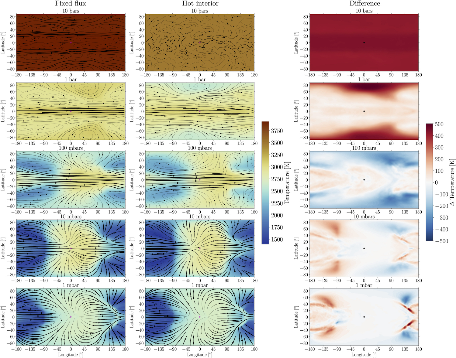
Figure 1: Maps of the hottest exoplanet in the model grid in the final 500 Earth days of the GCM simulation. The gradient colouring highlights the local temperature across the latitudes and longitudes of the atmosphere, while the arrows illustrate the circulation patterns in the atmosphere. Each row shows the temperature map at a different pressure depth within the atmosphere, with the deep interior at the top of the plot and the upper atmosphere at the bottom. On the left, the GCM results for the fixed flux version are shown, while the GCM results for the hot interior version are shown in the centre. On the right, the difference between the two setups at each pressure depth is shown. [Komacek et al. 2022]
What Does This Mean for Other Exoplanets?
Expanding their studies across the whole model grid, the authors find that similar patterns in the atmospheric dynamics are seen for all the orbital radii and surface gravities considered. There are, however, some differences between the impacts at low and high gravities. The hot-interior GCM leads to differences in atmospheric temperature of up to 10% compared to the fixed flux GCM for the lowest gravity case, while the high-gravity case sometimes leads to temperature differences of more than 20%.
With all the potential changes seen when considering a hot interior, particularly with differences occurring in the region probed by transmission spectroscopy, might the current standard “fixed flux” models make it harder to interpret these and similar observations? By observing exoplanets throughout their entire orbit in a phase curve, JWST is expected to constrain the pressure–temperature profiles of hot Jupiter atmospheres to tens of Kelvin. Given that the hot-interior GCM results differed in places by up to hundreds of Kelvin, it does indeed seem possible that such assumptions could be problematic.
Original astrobite edited by Katy Proctor.
About the author, Lili Alderson:
Lili Alderson is a PhD student at the University of Bristol studying exoplanet atmospheres with space-based telescopes. She spent her undergrad at the University of Southampton with a year in research at the Center for Astrophysics | Harvard-Smithsonian. When not thinking about exoplanets, Lili enjoys ballet, film and baking.


Cam So Far (but We Got So Far to Go)")


")


