Hunting Elusive SPRITEs with Spitzer
In recent years, astronomers have developed many wide-field imaging surveys in which the same targets are observed again and again. This new form of observing has allowed us to discover optical and radio transients — explosive or irregular events with durations ranging from seconds to years. The dynamic infrared sky, however, has remained largely unexplored … until now.
Infrared Exploration

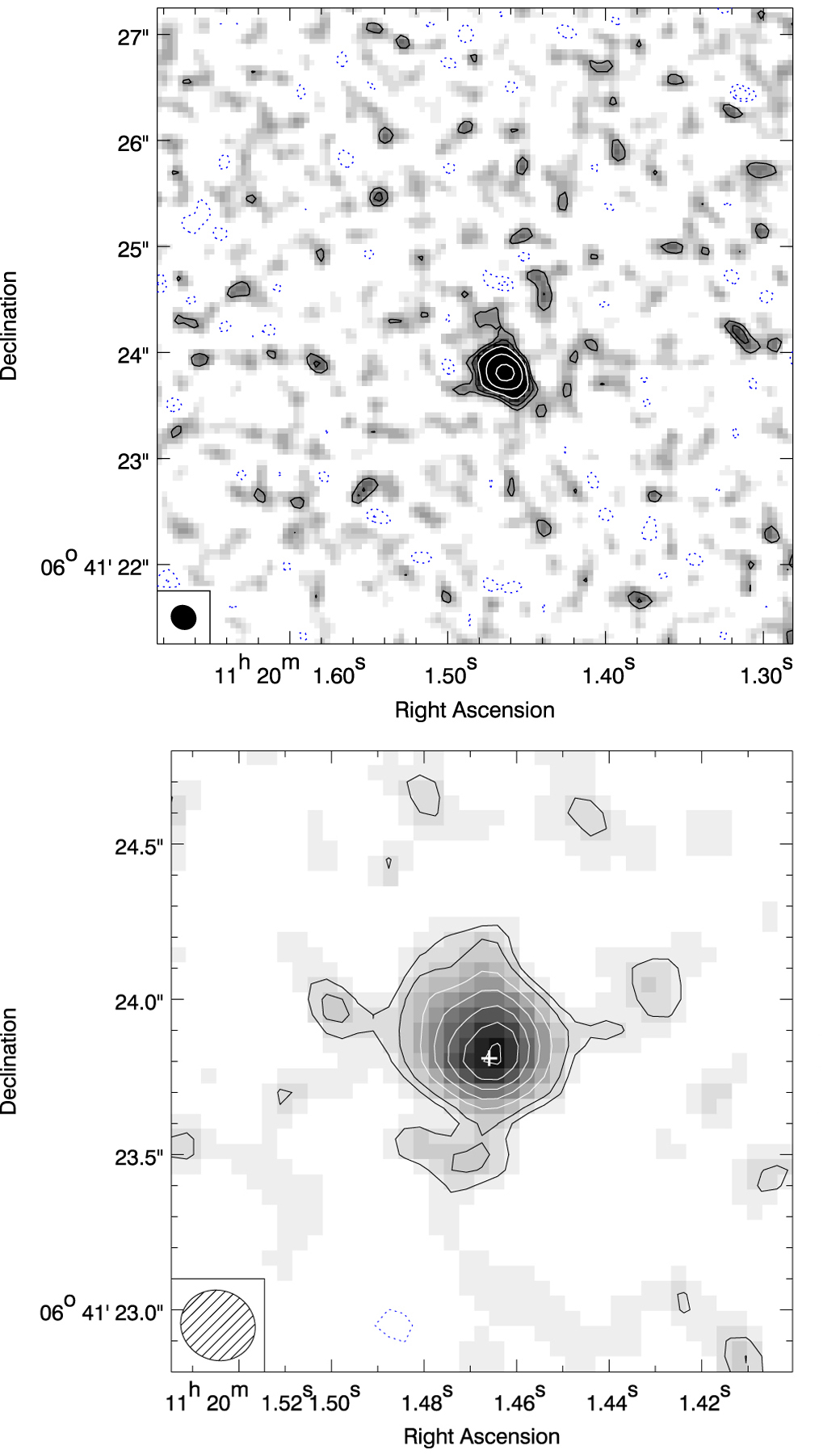
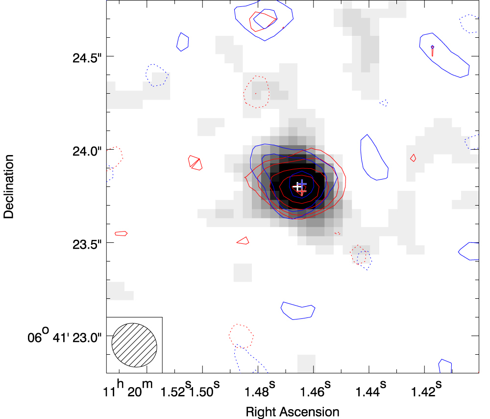
Example of a transient: SPIRITS 14ajc was visible when imaged by SPIRITS in 2014 (left) but it wasn’t there during previous imaging between 2004 and 2008 (right). The bottom frame shows the difference between the two images. [Adapted from Kasliwal et al. 2017]
To explore this uncharted territory, a team of scientists developed SPIRITS, the Spitzer Infrared Intensive Transients Survey. Begun in 2014, SPIRITS is a five-year long survey that uses the Spitzer Space Telescope to conduct a systematic search for mid-infrared transients in nearby galaxies.
In a recent publication led by Mansi Kasliwal (Caltech and the Carnegie Institution for Science), the SPIRITS team has now detailed how their survey works and what they’ve discovered in its first year.
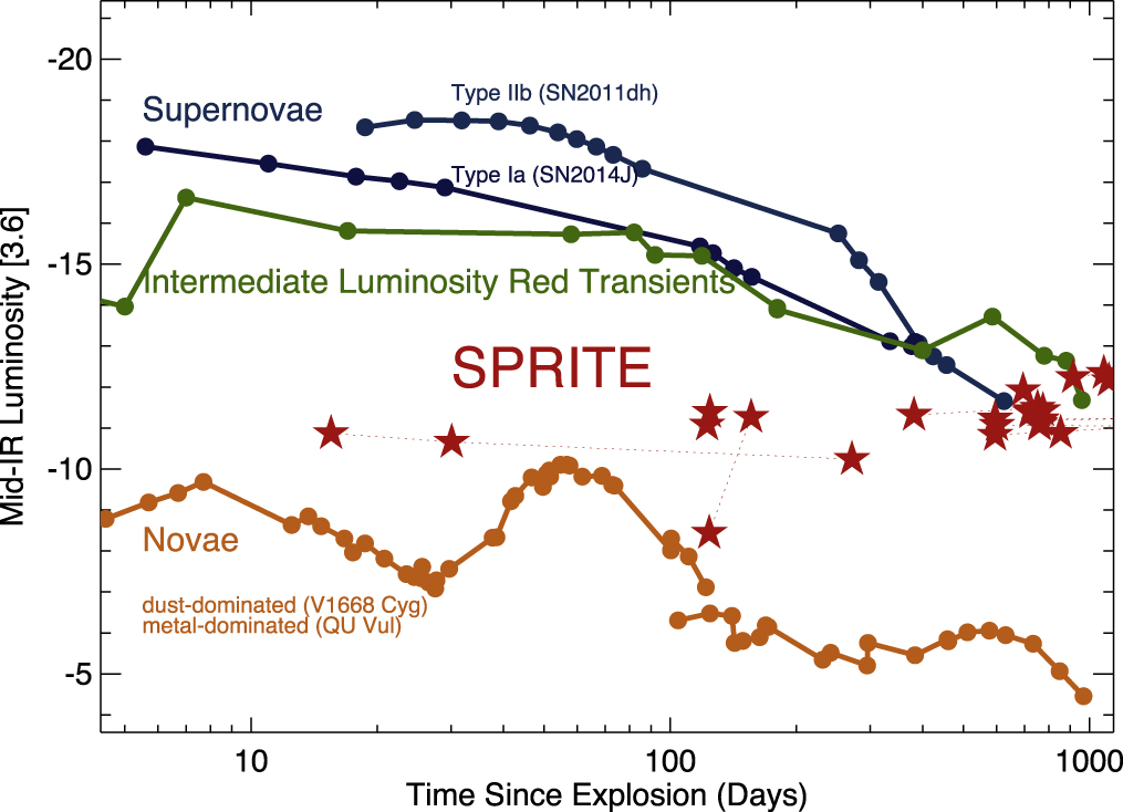
The light curves of SPRITEs (red stars) lie in the mid-infared luminosity gap between novae (orange) and supernovae (blue). [Kasliwal et al. 2017]
Mystery Transients
Kasliwal and collaborators used Spitzer to monitor 190 nearby galaxies. In SPIRITS’ first year, they found over 1958 variable stars and 43 infrared transient sources. Of these 43 transients, 21 were known supernovae, 4 were in the luminosity range of novae, and 4 had optical counterparts. The remaining 14 events were designated “eSPecially Red Intermediate-luminosity Transient Events”, or SPRITEs.
SPRITEs are unusual infrared transients that lie in the luminosity gap between novae and supernovae, and they have no optical counterparts. They all occur in star-forming galaxies.
Search for the Cause
What’s the physical origin of these phenomena? The authors explore a number of possible sources, including obscured supernovae, stellar mergers with dusty winds, collapse of extreme stars, or even weak shocks in failed supernovae.

Spitzer image of M83, one of the closest barred spiral galaxies in the sky. SPIRITS 14ajc was discovered in one of M83’s spiral arms. [NASA/JPL-Caltech]
The other SPRITEs may all have different origins, however, and in general the infrared photometric data isn’t sufficient to identify which model fits each transient. Future technology, like spectroscopy with the James Webb Space Telescope, may help us to better understand the origins of these elusive transients, though. And future surveying with projects like SPIRITS will help us to discover more SPRITE-like events, expanding our understanding of the dynamic infrared sky.
Citation
Mansi M. Kasliwal et al 2017 ApJ 839 88. doi:10.3847/1538-4357/aa6978


![Top: ALMA 1.3-mm observations of Elias 2-27’s spiral arms, processed with an unsharp masking filter. Two symmetric spiral arms, a bright inner ellipse, and two dark crescents are clearly visible. Bottom: a deprojection of the top image (i.e., what the system would look like face-on). [Meru et al. 2017]](https://aasnova.org/wp-content/uploads/2017/04/fig2-1.png)
![Left: Synthetic ALMA observations of disks shaped by an internal companion (top), an external companion (middle), and gravitational instability within the disk (bottom). Right: Deprojections of the images on the left. Scale is the same as in the actual observations above. The external companion and the gravitational instability scenarios match the actual ALMA observations of Elias 2-27 well. [Adapted from Meru et al. 2017]](https://aasnova.org/wp-content/uploads/2017/04/fig3_vertical-1.png)