Another Possibility for Boyajian’s Star
The unusual light curve of the star KIC 8462852, also known as “Tabby’s star” or “Boyajian’s star”, has puzzled us since its discovery last year. A new study now explores whether the star’s missing flux is due to internal blockage rather than something outside of the star.
Mysterious Dips
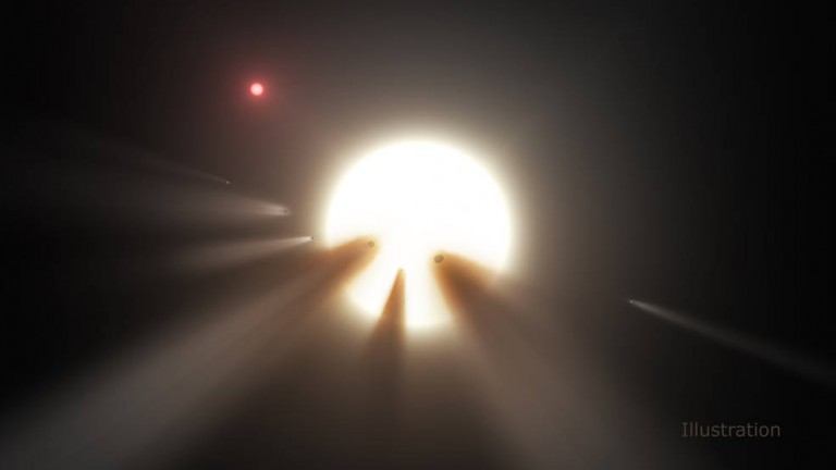
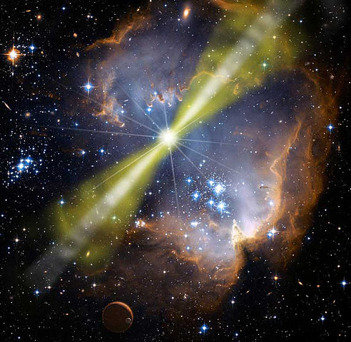
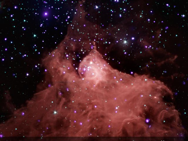
Most explanations for the flux dips of Boyajian’s star rely on external factors, like this illustrated swarm of comets. [NASA/JPL-Caltech]
Explanations thus far have varied from mundane to extreme. Alien megastructures, pieces of smashed planets or comets orbiting the star, and intervening interstellar medium have all been proposed as possible explanations — but these require some object external to the star. A new study by researcher Peter Foukal proposes an alternative: what if the source of the flux obstruction is the star itself?
Analogy to the Sun
Decades ago, researchers discovered that our own star’s total flux isn’t as constant as we thought. When magnetic dark spots on the Sun’s surface block the heat transport, the Sun’s luminosity dips slightly. The diverted heat is redistributed in the Sun’s interior, becoming stored as a very small global heating and expansion of the convective envelope. When the blocking starspot is removed, the Sun appears slightly brighter than it did originally. Its luminosity then gradually relaxes, decaying back to its original value.
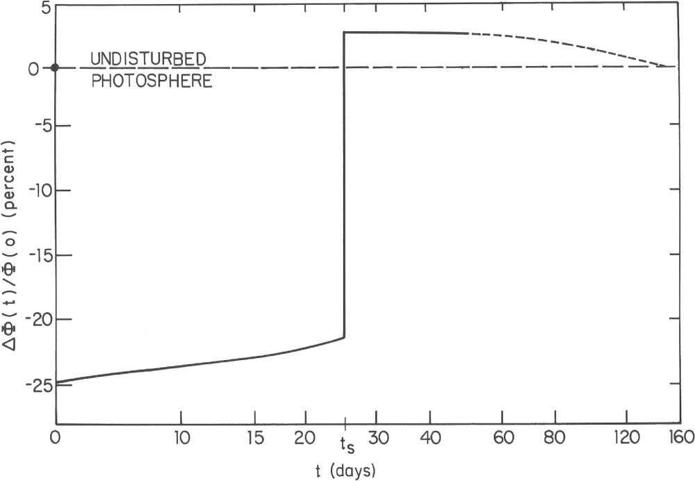
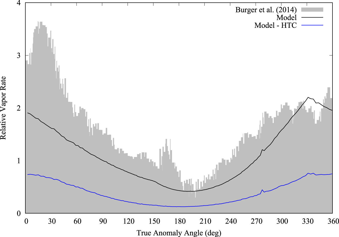
Model of a star’s flux after a 1,000-km starspot is inserted at time t = 0 and removed at time t = ts at a depth of 10,000 km in the convective zone. The star’s luminosity dips, then becomes brighter than originally, and then gradually decays. [Foukal 2017]
In addition, these sporadic flux-blocking events would cause Boyajian’s star to constantly be relaxing from the post-blockage enhanced luminosity. This decay — which occurs at rates of 0.1–1% brightness per year for convective-zone depths of tens of thousands of kilometers — would nicely account for the long-term, gradual dimming observed.
What’s blocking the flux? Foukal postulates a few options, including magnetic activity (as with the Sun), differential rotation, sporadic changes in photospheric abundances, and simply random variation in convective efficiency.
Strangely Unique
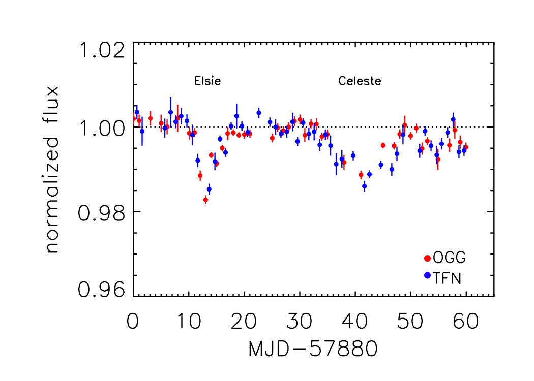
Boyajian’s star’s flux in May and June shows some brand new dips. Note that the team now names them! [Tabetha Boyajian and team]
Until we discover more cases, the best we can hope for is more data from Boyajian’s star itself. Conveniently, it has continued to keep us on our toes, with new dips in May and June. Perhaps our continued observations will finally reveal the answer to this mystery.
Citation
Peter Foukal 2017 ApJL 842 L3. doi:10.3847/2041-8213/aa740f