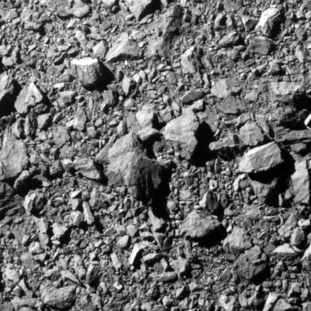
The final full image from DART, taken 2 seconds before the spacecraft crashed into the asteroid moonlet Dimorphos. [NASA/Johns Hopkins APL]
In 2022, humanity performed its first test of its ability to defend itself against an oncoming asteroid impact. When NASA’s Dual Asteroid Redirection Test (DART) spacecraft slammed into Dimorphos, the 160-meter-wide moonlet of the asteroid Didymos, a spray of material escaped the moonlet’s surface, and Dimorphos’s path around its parent asteroid was altered — showing how a 610-kilogram spacecraft can change the course of a 4.8-
billion-kilogram asteroid. Both the spray of ejecta and the change in orbit reflect the transfer of momentum from the spacecraft, which came in at a screaming 22,530 kilometers per hour.
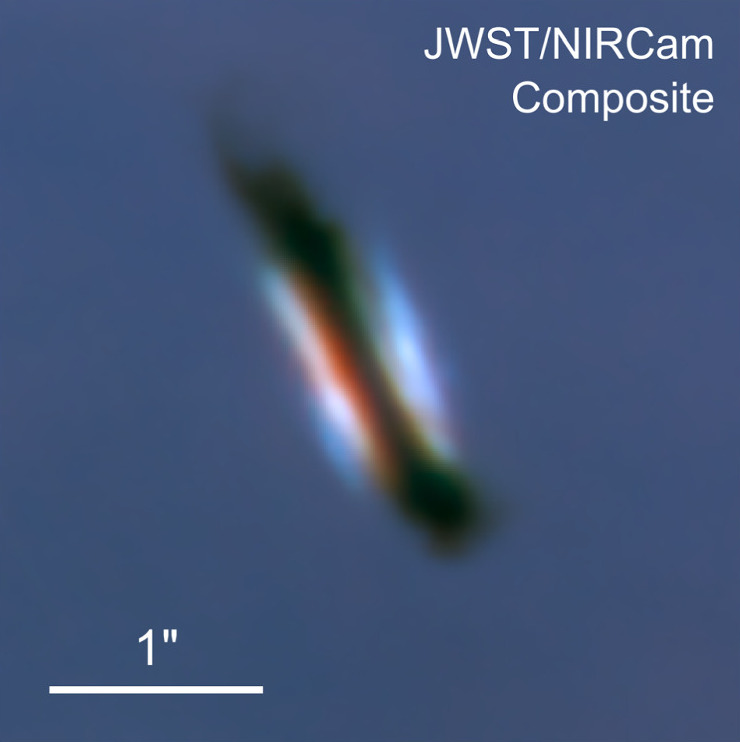
Could an impact from a spacecraft like DART actually nudge a hazardous asteroid onto a safer course? The timeliness of this question recently ratcheted up a notch: the probability of the asteroid 2024 YR4 striking Earth on 22 December 2032 has risen above 2%.
Discovery images of 2024 YR4. [ATLAS]
Answering this question isn’t straightforward. Among the factors that influence the outcome of a mission like DART — or a future mission to reshape the trajectory of a hazardous asteroid — is the target asteroid’s structure and material strength. Today, we’re taking a look at three research articles that tackle simulations of an impactor striking an asteroid to understand the role of asteroid structure and strength, providing results relevant to both planetary defense and the study of asteroid properties.
Subsurface Structure and Impact Outcomes
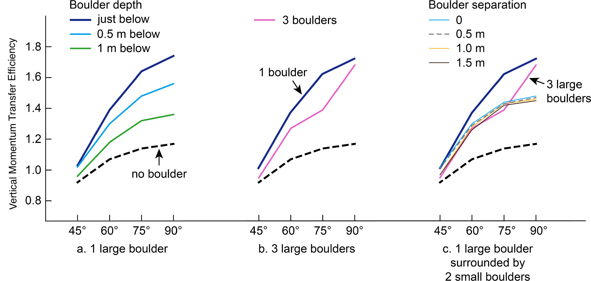
First up, a team led by Kaiyi Dai (Macau University of Science and Technology; Imperial College London) and Xi-Zi Luo (Macau University of Science and Technology) simulated the outcome of an impactor striking an asteroid at an angle, just as DART did, rather than head on. Their goal was to understand how the presence of boulders — like those expected to make up “rubble-pile” asteroids like Didymos and Dimorphos — affects the transfer of momentum from the impactor to the target asteroid. Specifically, the team used a three-dimensional shock physics code to explore the effect of different subsurface arrangements of boulders.
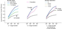
Momentum transfer efficiency as a function of the impact angle for different boulder configurations. Click to enlarge. [Adapted from Dai et al. 2024]
An impactor striking a rubble-pile asteroid doesn’t just dislodge material: it also melts some of it. The simulations showed that the amount of melted material, as well as whether the melted material remained on the surface or was ejected into space, varied substantially with the angle of the impact and the configuration of subsurface boulders. This suggests that the volume of melted material remaining on an asteroid’s surface could be used to discern the structure of the material beneath the surface.
Dai and Luo’s team noted that applying these simulation results to the outcome of the DART mission will require simulating a more realistic impactor, as the DART spacecraft’s shape and composition is more complicated than that of the spherical projectile used in these simulations.
Impact of Asteroid Strength and Porosity
Mallory DeCoster (Johns Hopkins University Applied Physics Laboratory) and collaborators also investigated the outcomes of high-velocity impacts on rubble-pile asteroids. The team focused on the effects of not only the boulders at the impact site, but also the “matrix material” of finer particles between the boulders. Because this matrix material effectively holds a rubble-pile asteroid together, the strength of the material plays a large role in determining the outcome of an impact.
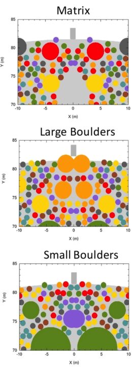
Examples of matrix, large boulder, and small boulder configurations. Matrix material is shown as gray, the impactor is the small gray rectangle, and boulders are shown in different colors (the color of the boulder does not have any meaning). [Adapted from DeCoster et al. 2024]
The team carried out 52 two-dimensional shock physics simulations of impacts onto an asteroid that is 163 meters across — roughly the size of Dimorphos. The properties of the impactor were tuned to be similar to the DART spacecraft: a porous aluminum cylinder 2 meters long and 0.5 meter wide with a mass of 501 kilograms and an impact velocity of 6.6 kilometers per second. The porosity of the simulated cylinder reflects the fact that spacecraft aren’t solid, and this porosity changes the way the impactor interacts with the target.
DeCoster and collaborators placed boulders with diameters of 1–10 meters randomly within their simulated asteroids, filling 62% of each asteroid with boulders before topping off the rest of the volume with matrix material. The simulated asteroids were categorized as “matrix,” “large boulders,” and “small boulders” depending on the primary makeup of the impact site. The strength and porosity of the matrix material were varied between simulations.
The simulations showed that more porous matrix material resulted in larger impact craters, but this outcome was moderated by the distribution of boulders on and under the surface; for matrix-rich asteroids, the presence of weaker, more porous material boosted the crater width, while asteroids with many large or small boulders showed smaller differences in crater width with matrix strength and porosity. None of these factors particularly influenced the depth of the crater.
Matrix-rich asteroids tended to experience larger momentum transfer than boulder-rich asteroids, but this finding was complicated by certain boulder-rich simulations in which entire boulders were thrown into space, resulting in a large momentum transfer for those simulation runs. These results highlight the complex factors that determine how an asteroid responds to an impact.
Estimating Cratering on Dimorphos
The final of today’s three research articles focuses on simulations of the DART spacecraft impacting Dimorphos. After DART slammed into the asteroid, the Italian Space Agency’s Light Italian CubeSat for Imaging of Asteroids (LICIACube) surveyed the aftermath from a safe distance. LICIACube imaging showed fantastic sprays of ejecta and boulders tumbling through space, but the precise size of the crater excavated by DART’s impact is still unknown. That will change with the arrival of the European Space Agency’s Hera mission, which launched in October 2024. Upon reaching Dimorphos and Didymos in late 2026, Hera will assess the impact site and measure the size of the impact crater.
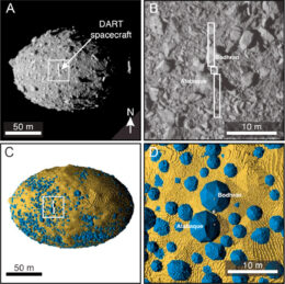
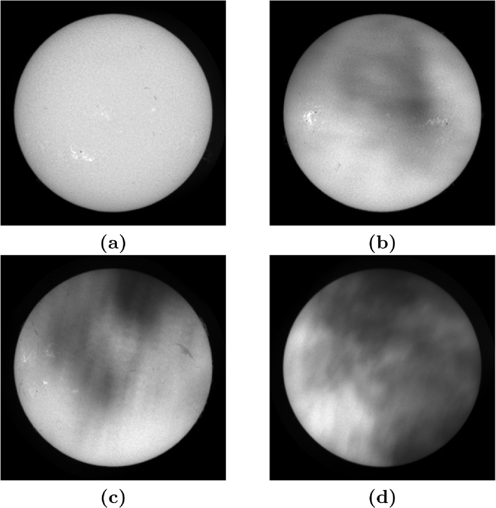
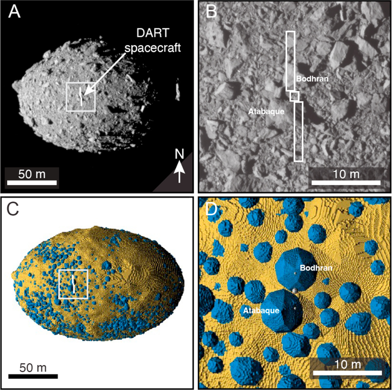
DART observations of Dimorphos before impact (panels a and b). Panels c and d show the rubble-pile target constructed to match the DART observations. Click to enlarge. [Stickle et al. 2025]
While they wait for Hera to finish its journey, scientists are fine-tuning their simulations. Angela Stickle (Johns Hopkins University Applied Physics Laboratory) and collaborators used information gleaned from the DART mission — namely, the change in Dimorphos’s orbit, the characteristics of the ejecta, and the appearance of the asteroid’s surface — to predict the size of the resulting crater.
Stickle’s team modeled Dimorphos as a collection of boulders held together by matrix material, with the sizes and positions of the surface boulders determined from pre-impact photographs of the asteroid. The sizes of the subsurface boulders were drawn from the same size–frequency distribution as observed for the surface boulders, and these boulders were given random non-spherical shapes. The impactor was a DART-like conglomeration of three spheres, with the large central sphere representing the body of the spacecraft and two smaller, lower-mass side spheres representing the spacecraft’s solar panels.
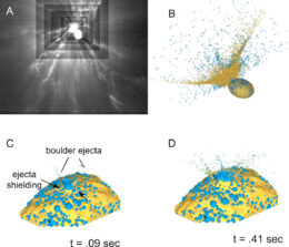
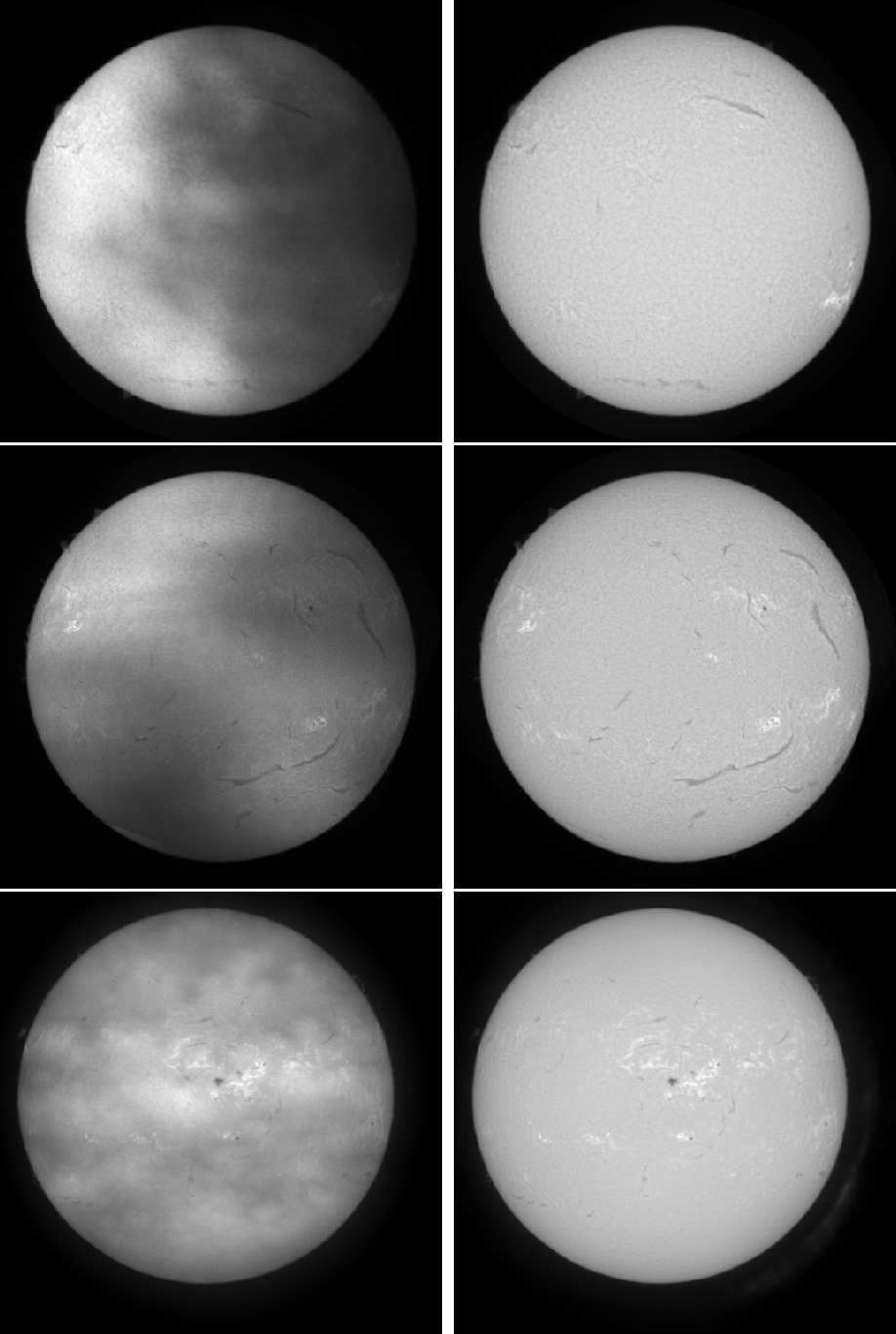
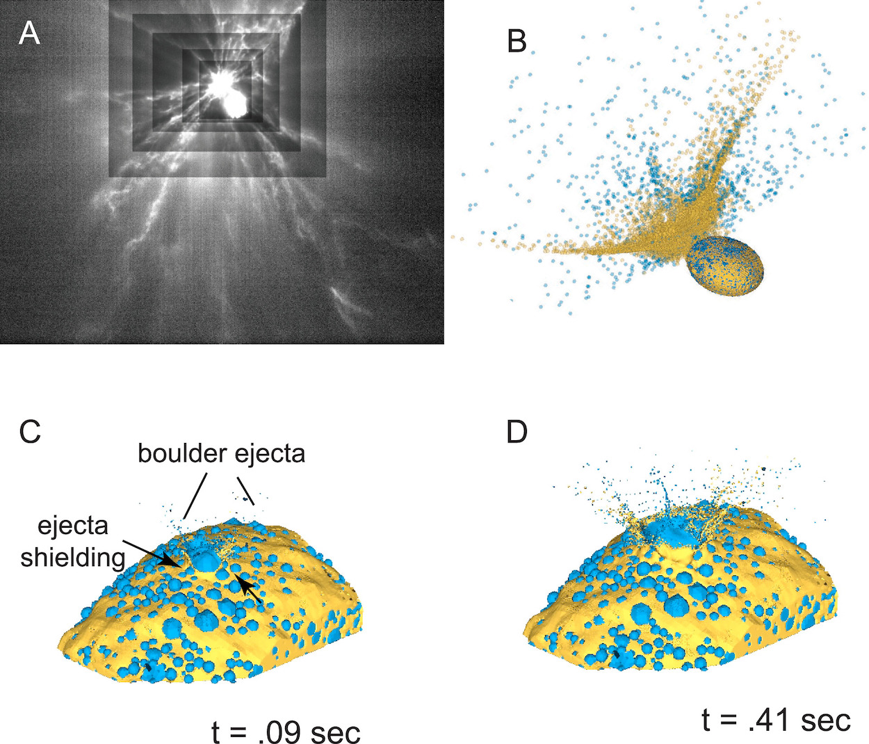
Comparison of LICIACube observations of ejecta rays (panel a) to simulated ejecta (panels b through d). Click to enlarge. [Stickle et al. 2025]
Using three shock physics codes, Stickle’s team examined the transfer of momentum, the creation of a crater, and the production of filamentary ejecta rays like those seen by LICIACube. A rubble-rich structure seems to be necessary to create dramatic ejecta rays, supporting the classification of Dimorphos as a rubble-pile asteroid.
The transfer of momentum — a marker of the ability of an impactor to deflect the asteroid from its initial trajectory — depended strongly on the material properties of the asteroid: less-cohesive asteroid material with a larger resistance to crushing correlated with larger momentum transfer.
Estimated crater diameters ranged from 15 to 60 meters, with the likeliest size for Dimorphos being in the range of 40–60 meters. The team notes that this calculation is complicated, as crater sizes continue to evolve beyond the end of the simulations in a way that depends on the strength of the material and the gravity of the asteroid.
The upcoming measurements from the Hera mission will provide an important test of these model results, providing further information on the outcome of the DART mission and helping to advance our understanding of humanity’s ability to deflect hazardous asteroids.
Citation
“Impact Momentum Transfer — Insights from Numerical Simulation of Impacts on Large Boulders of Asteroids,” Kaiyi Dai et al 2024 Planet. Sci. J. 5 214. doi:10.3847/PSJ/ad72eb
“Statistical Analysis of Near-Surface Structure and Material Properties on Momentum Transfer in Rubble Pile Targets Impacted by Kinetic Impactors,” Mallory E. DeCoster et al 2024 Planet. Sci. J. 5 244. doi:10.3847/PSJ/ad7cff
“Dimorphos’s Material Properties and Estimates of Crater Size from the DART Impact,” Angela M. Stickle et al 2025 Planet. Sci. J. 6 38. doi:10.3847/PSJ/ad944d