Features RSS

Titan's seas

The frigid seas of Titan, Saturn’s largest moon, host a secret: something is causing features to appear and disappear within them. Could these seas be bubbling? And if so, how could such bubbles form and grow?

Frigid Seas

Titan

Near-infrared mosaic showing sunlight reflecting off of Titan’s north polar hydrocarbon seas. [NASA/JPL-Caltech/University of Arizona/University of Idaho]

While observing Saturn’s rings in 1655 — that’s a whopping 363 years ago! — Dutch astronomer Christiaan Huygens spotted something else: Saturn’s largest moon, Titan. In 2007, more than three centuries later, we got our first up-close look at Titan when the Cassini/Huygens probe arrived at Saturn and discovered new surprises from this moon.

Titan is a hostile, chilly world, with a nitrogen atmosphere and an icy crust. Its distance from the Sun is roughly ten times the Earth–Sun distance, so Titan’s surface temperatures are only around 95 K (–290 °F). At this temperature, hydrocarbons methane and ethane take liquid form, pooling in pockets in Titan’s crust to form hundreds of hydrocarbon lakes and seas that dot Titan’s surface.

magic islands in Ligeia Mare

Evolution of transient bright features — “magic islands” — in Ligeia Mare, as seen by radar images. Click for a better look. [NASA/JPL-Caltech/ASI/Cornell]

Magic Islands

In the past few years, scientists have noticed something odd about one of these seas, the northern Ligeia Mare: radar observations of Titan’s surface have shown bright regions within the sea that appear and vanish from one flyby to the next. In acknowledgement of these features’ mysteriousness, scientists nicknamed them “magic islands”.

What could be causing these transient features? One of the more popular explanations is that streams of bubbles are being released as atmospheric nitrogen — originally dissolved in the liquid methane and ethane of the sea — separates out and rises to the surface.

Now, two scientists from the University of Reims Champagne-Ardenne in France, Daniel Cordier and Gérard Liger-Belair, want to understand whether such bubbles could even form in the unique environment of Titan’s seas.

Growing Bubbles from the Seafloor

Cordier and Liger-Belair start their study from what we know: if the “magic islands” are, in fact, bubbles, then they must be at least ~2cm in size near the surface of Ligeia Mare; if they were any smaller, they wouldn’t reflect the radar waves. The authors then use theoretical calculations and simulations to explore ways to form and grow bubbles to this size in a hydrocarbon sea.

bubble column schematic

Authors’ sketch of a column of bubbles within Titan’s liquid methane/ethane seas. Radar waves come in from above and reflect off of the bubbles. [Cordier & Liger-Belair 2018]

Cordier and Liger-Belair find that homogeneous nucleation, where bubbles form without a surface, can’t explain the observations under the conditions of Titan’s surface. But heterogeneous nucleation, in which bubbles form on surfaces like the seabed or suspended sediment particles, can work to produce bubbles that grow to reach ~2-cm sizes.

The authors show that the best explanation for large bubbles at Ligeia Mare’s surface is that bubbles form or are released tens of meters down at the seabed and then rise as a vertical column. As the bubbles bump into each other and combine within this plume, they arrive at the sea’s surface at a potential size perfect for reflecting radar waves.

Cordier and Liger-Belair’s work shows that nitrogen bubbles in a methane and ethane sea could indeed explain the “magic islands” we only discovered after three centuries of studying Titan. Who knows what we’ll learn in the next three centuries observing this mysterious moon!

Citation

Daniel Cordier and Gérard Liger-Belair 2018 ApJ 859 26. doi:10.3847/1538-4357/aabc10

Magellanic Clouds

The Magellanic Clouds — two nearby dwarf galaxies easily visible to the naked eye in the southern hemisphere — are key to understanding the dynamics and evolution of the Local Group of galaxies. Can an in-depth look at these galaxies’ outer regions help us make sense of their complicated interaction history?

A Closer Look at Our Galactic Neighbors

Magellanic Stream

A combined optical and radio view of the Milky Way and the Magellanic Stream, shown in pink. [David L. Nidever, et al., NRAO/AUI/NSF and Mellinger, Leiden/Argentine/Bonn Survey, Parkes Observatory, Westerbork Observatory, and Arecibo Observatory]

The Small and Large Magellanic Clouds (SMC and LMC) have been well studied, but these dwarf satellite galaxies continue to inspire new discoveries. Among them is the origin of the Magellanic Stream — a swath of neutral hydrogen trailing the Magellanic Clouds and spanning more than half a million light-years.

It was originally thought that the Magellanic Stream was the result of tidal interactions during close encounters with the Milky Way, but precise proper motion surveys revealed that the LMC and SMC are either passing near the Milky Way for the first time or are in a long (~4-billion-year) orbit around our galaxy — so the Magellanic Stream must result from interactions between the two galaxies themselves.

How long have the LMC and SMC been interacting, and how have these interactions shaped the two galaxies? A key to understanding the history of these dwarf galaxies is mapping the weakly gravitationally bound stars at their far edges that may be pulled into tidal streams or bulges as each galaxy is distorted by the presence of the other.

Stellar substructures

A map of the density of ancient stars surrounding the Magellanic Clouds reveals extended structures to the north and south of the LMC, while the western regions of the galaxy (to the right) are truncated. Click to enlarge. [Adapted from Mackey et al. 2018]

Mapping the Edges of Galaxies

Dougal Mackey (Australian National University) and collaborators used visible and near-infrared images taken by the Dark Energy Camera (DECam) — the workhorse instrument of the Dark Energy Survey — to map the faint outskirts of the LMC and SMC.

Though the purpose of the Dark Energy Survey is to better understand the nature of dark energy through observations of supernovae, weak gravitational lenses, and galaxy clusters, its sensitive imaging system and wide field of view (2.2 degrees in diameter) make it well-suited to exploring the faint fringes of nearby galaxies.

The DECam images of the Magellanic Clouds probed to a surface brightness of 32 magnitudes per square arcsecond, allowing Mackey and collaborators to investigate how different stellar populations are distributed in the outer regions of these galaxies.

Stellar population maps

Stellar density maps for young (<1 Gyr) and intermediate-age (1.5–4 Gyr) populations. The young stars trace a bridge between the galaxies, while the intermediate-age stars are offset from the ancient stars in the direction of the LMC. Click to enlarge. [Adapted from Mackey et al. 2018]

Structures Revealed in Faint Starlight

Mapping the density of stars revealed distinct stellar substructures on the outskirts of the LMC and SMC. While previous studies discovered isolated substructures on the outer limits of the LMC, the panoramic view from this study highlights the interconnected nature of the structures.

One important finding is that the intermediate-age (1.5–4 Gyr) stellar population of the SMC is distinctly offset from the ancient (~11 Gyr) stellar population. This result suggests that the Magellanic Clouds may have been gravitationally linked as far back as several billion years — hinting that these galaxies are on their first trip past the Milky Way. Future simulation work may provide a more cohesive picture of the LMC–SMC interaction, helping us better understand how our near neighbors have evolved.

Citation

Dougal Mackey et al 2018 ApJL 858 L21. doi:10.3847/2041-8213/aac175

protoplanetary disk

What’s one thing the interstellar medium, protoplanetary disks, stellar interiors, and the environments around black holes all have in common? They all contain dust grains moving within a fluid — and two scientists from the California Institute of Technology say we’ve been missing an important part of their behavior.

Pairing of Fluids and Dust

Crab Nebula

Hubble view of the Crab Nebula. Supernova ejecta are another instance of a coupled system of dust grains and fluid. [NASA/ESA/J. Hester and A. Loll (Arizona State University)]

Fluids — which can refer to liquids, gases, or plasmas — rarely exist in isolation in astrophysics. More often than not, fluids come laden with dust particles; examples of dusty fluids include the environments near star-forming regions, in planetary atmospheres, in the disks surrounding young stars, or even around active galactic nuclei. Since these fluid/dust systems are abundant across the universe and are fundamental to many key astrophysical processes, it’s important that we understand how they behave.

Caltech scientists Jonathan Squire and Philip Hopkins ask one particular question: what happens when dust particles move at a different speed than the fluid surrounding them?

Relative Motion

Relative motion of dust through fluid can arise naturally through many mechanisms. Radiation pressure, for instance, preferentially accelerates dust grains relative to gas in environments around active galactic nuclei or in the envelopes of stars, causing the dust to stream through the surrounding fluid. Or the fluid of a planetary atmosphere might be supported against gravity by thermal pressure, causing the heavier dust grains to settle downward through the fluid.

In a new study, Squire and Hopkins suggest that this relative streaming motion between dust grains and fluid can easily create instabilities — and this can have profound implications for our understanding of many fields of astrophysics.

Instabilities Found Everywhere

The authors used analytic calculations to show that coupled fluid/dust systems can develop “resonant drag instabilities” whenever the dust grains stream faster than any wave in the fluid.

planetary atmosphere

In a planetary atmosphere like the one shown in this artist’s impression, a fluid might be supported against gravity, whereas dust grains are not. This would create relative motion of the dust particles as they settle. [Max Planck Society]

These instabilities, it turns out, are quite easy to trigger, because astrophysical fluids host a variety of waves, any of which can form the basis for a resonant drag instability. Examples include sound waves, magnetosonic waves, Brunt–Väisälä waves, epicyclic oscillations, and others. The instabilities triggered by the streaming dust in the presence of these waves grow over time, causing spatial clumping of the dust and eventually seeding turbulence if they’re strong enough.

Squire and Hopkins present a way of calculating the growth rates and properties of these resonant drag instabilities in different fluids, and they demonstrate the behavior of the instabilities in three example fluid systems: hydrodynamic, magnetohydrodynamic, and stratified fluids.

The authors argue that the consequences of the resonant drag instability affect regions and processes like planetesimal formation, cool-star winds, active galactic nuclei torii and winds, starburst regions, H II regions, supernovae ejecta, and the circumgalactic medium. Their work toward understanding this instability is therefore broadly applicable across astronomical fields, providing critical insight into processes in our universe.

Citation

J. Squire and P. F. Hopkins 2018 ApJL 856 L15. doi:10.3847/2041-8213/aab54d

Screenshot of the user interface for WWT shows clusters of objects plotted against a sky background.

One of the most rapidly evolving elements of astronomy research is how we handle data. With telescopes and computer simulations progressively producing ever vaster quantities, how can we process and analyze this data? What tools can we use to turn it into new astronomical discoveries?

The future of astronomy relies on new innovations on this front, and in a Special Issue of the Astrophysical Journal Supplement Series, 23 papers explore different insights and challenges related to astronomical data — presenting new workflows, software instruments, databases, and tutorials that will aid astronomers in generating novel and significant research results.

Here are the broad categories of data in astronomy that are touched on in this special issue:

volume renderings

Volume renderings from a simulation of a low metallicity star. This is an example of the data that can be analyzed using cyberhub, a web-browser-based tool for medium-sized collaborations. [Herwig et al. 2018]

1. Cloud-Based Research Environments for Discovery

Collaborations in astronomy are often large and broadly distributed. As a result, the astronomy community needs the infrastructure to be able to access large data sets, combine them, and collaboratively process them to make discoveries. An article by Herwig et al. presents the cyberhubs system, a package for medium-sized scientific teams to collaboratively interact with data via web browser. Williams et al. discuss the challenges inherent in reducing a large photometric data set — in their case, data from the Panchromatic Hubble Andromeda Treasury (PHAT) — on the Amazon Elastic Compute Cloud (EC2), a commercial system of virtual computers that users can rent on demand. Heidorn et al. present Astrolabe, a cyberinfrastructure project of the University of Arizona and the American Astronomical Society that aims to ensure the long-term curation of astronomical data for future reference and use.

2. Software Instruments for Transient Detection, Alerts, and Analysis

time-variable sources

Just some of the time-variable sources that are detected and analyzed, and their characteristic timescales for variation. [Narayan et al. 2018]

Given the current boom of time-domain astronomy, the development of tools for studying transient astronomical phenomena is crucial. Necessary tools include not only those that will detect transients, but also those that provide alerting for rapid followup, and those that enable analysis of the large quantities of resulting data. Law et al. discuss realfast, a fast transient search system at the Jansky Very Large Array that will look for transients in real time as data comes in, reducing the amount of data that must be stored. Guillochon et al. introduce MOSFiT, a software package that enables rapid comparison of transient data to models. And Narayan et al. present ANTARES, an automated software system that sifts through, characterizes, annotates, and prioritizes transient events for followup, allowing for rapid alerting of the community to transients that warrant additional observations.

In addition to searching for unexpected transient events, time-domain astronomers also study the variability of single sources. He et al. describe a long-term study of magnetic-feature and flare activity of three Sun-like stars with Kepler. As for the Sun itself — studying it in detail produces terabytes-per-hour streams of data that must be captured and analyzed. Denker et al. present the challenges of managing such a stream of high-resolution observations at the GREGOR Solar Telescope, and Boubrahimi et al. explore how best to interpolate between solar data collected from a variety of ground-based and space-based solar observatories every day.

3. Statistical Properties of Data with Uncertainties or Gaps

How do we address the issue of incomplete or uncertain data? Correct application of statistical methods are an important aspect of data reduction. Hogg et al., Vianello, Huppenkothen et al., VanderPlas, Huijse et al., Ma et al., and Aggarwal et al. all present on methods of careful statistical handling of astronomical data — covering topics from an overview of Markov Chain Monte Carlo methods for sampling probability density functions, to a look at how we might use statistics to predict solar eruptions.

OSSOS TNOs

Blue dots represent the 838 characterized OSSOS discoveries of trans-Neptunian objects from a recent data release. [Bannister et al. 2018]

4. New Database Releases

The production of vast amounts of data isn’t enough — it must also be compiled in a useful way before it can be analyzed by the community. The regular release of large, updated databases are an important driver of astronomical discovery. In this Special Issue, Bannister et al. present the Outer Solar System Origins Survey (OSSOS), a data release of more than 800 trans-Neptunian objects, and Egeland introduces sunstardb, a database useful for studying stars in analogy to the Sun.

5. Astronomy Data in Publication

The big-data boom produces many important questions in scientific publishing, like how data will be cited and classified, whether software instrument source codes will be made available, and what impact these references might have on the future of astronomical publication. Novacescu et al. discuss the policy of data citation — in particular, using digital object identifiers (DOIs) to refer to data both analyzed and generated by research projects. Frey et al. present an update on the Unified Astronomy Thesaurus, an effort to unite astronomers under a single vocabulary to govern keywords and classification for astronomy research. Allen et al. address the issue of source code availability: can other researchers easily access the software you used, to explore or reproduce your results? Varga examines how metrics based on references or keywords can be used to predict citation impact for scientific articles.

6. Advances in Data Visualization

WWT UI

More screen captures of the WorldWide Telescope user interface. [Rosenfield et al. 2018]

One challenge of astronomy data echoes the challenge inherent in all of science: how can we best communicate and share it? Rosenfield et al. introduce a tool for this, the American Astronomical Society’s WorldWide Telescope (WWT). This project enables terabytes of astronomical images, data, and stories to be viewed and shared among researchers, exhibited in science museums, projected into full-dome immersive planetariums and virtual reality headsets, and taught in classrooms.

It’s evident that there are indeed many challenges raised by the production and management of vast amounts of astronomical data — but there are also many opportunities available. The articles in this Special Issue are meant to provide an introduction to some of the topics currently under consideration, but conversations will continue to evolve as we adapt to this age of big data.

Citation

Special ApJS Issue on Data

Frank Timmes and Leon Golub 2018 ApJS 236 1. doi:10.3847/1538-4365/aab770

black holes in a globular cluster

What is the distribution of sizes of black holes in our universe? Can black holes of any mass exist, or are there gaps in their possible sizes? The shape of this black-hole mass function has been debated for decades — and the dawn of gravitational-wave astronomy has only spurred further questions.

Mind the Gaps

The starting point for the black-hole mass function lies in the initial mass function (IMF) for stellar black holes — the beginning size distribution of black holes after they are born from stars. Instead of allowing for the formation of stellar black holes of any mass, theoretical models propose two gaps in the black-hole IMF:

  1. An upper mass gap at 50–130 solar masses, due to the fact that stellar progenitors of black holes in this mass range are destroyed by pair-instability supernovae.
  2. A lower mass gap below 5 solar masses, which is argued to arise naturally from the mechanics of supernova explosions.
Missing black-hole formation channels

Missing black-hole (BH) formation channels due to the existence of the lower gap (LG) and the upper gap (UG) in the initial mass function. a) The number of BHs at all scales are lowered because no BH can merge with BHs in the LG to form a larger BH. b) The missing channel responsible for the break at 10 solar masses, resulting from the LG. c) The missing channel responsible for the break at 60 solar masses, due to the interaction between the LG and the UG. [Christian et al. 2018]

We can estimate the IMF for black holes by scaling a typical IMF for stars and then adding in these theorized gaps. But is this initial distribution of black-hole masses the same as the distribution that we observe in the universe today?

The Influence of Mergers

Based on recent events, the answer appears to be no! Since the first detections of gravitational waves in September 2015, we now know that black holes can merge to form bigger black holes. An initial distribution of black-hole masses must therefore evolve over time, as mergers cause the depletion of low-mass black holes and an increase in higher-mass black holes.

A team of scientists led by Pierre Christian, a graduate student at Harvard University, has now looked into characterizing this shift. In particular, Christian and collaborators explore how black-hole mergers in the centers of dense star clusters ultimately shape the black-hole mass function of the universe.

Black Holes Today

Christian and collaborators use analytical models of coagulation — mergers of particles to form larger particles — to estimate the impact of mergers in star clusters on resulting black-hole sizes. They find that, over an evolution of 10 billion years, mergers can appreciably fill in the upper mass gap of the black-hole IMF.

black-hole mass function

An example of the black-hole mass function that can result from evolving the initial mass function — complete with gaps — over time. Two breaks appear as a result of the initial gaps: one at ~10 (LB) and one at ~60 solar masses (UB). [Christian et al. 2018]

The lower mass gap, on the other hand, leaves observable signatures in the final black-hole mass function: a break at 10 solar masses (since black holes below this mass can’t be created by mergers) and one at 60 solar masses (caused by the interaction of the upper and lower gaps). As we build up black-hole statistics in the future (thanks, gravitational-wave detectors!), searching for these breaks will help us to test our models.

Lastly, the authors find that their models can only be consistent with observations if ejection is efficient — black holes must be regularly ousted from star clusters through interactions with other bodies or as a result of kicks when they merge. This idea is consistent with many recent studies supporting a large population of free-floating stellar-mass black holes.

Citation

Pierre Christian et al 2018 ApJL 858 L8. doi:10.3847/2041-8213/aabf88

infrared galactic center

Finding planets in the crowded galactic center is a difficult task, but infrared microlensing surveys give us a fighting chance! Preliminary results from such a study have already revealed a new exoplanet lurking in the dust of the galactic bulge.

Detection Biases

UKIRT-2017 microlensing survey fields

UKIRT-2017 microlensing survey fields (blue), plotted over a map showing the galactic-plane dust extinction. The location of the newly discovered giant planet is marked with blue crosshairs. [Shvartzvald et al. 2018]

Most exoplanets we’ve uncovered thus far were found either via transits — dips in a star’s light as the planet passes in front of its host star — or via radial velocity wobbles of the star as the orbiting planet tugs on it. These techniques, while highly effective, introduce a selection bias in the types of exoplanets we detect: both methods tend to favor discovery of close-in, large planets orbiting small stars; these systems produce the most easily measurable signals on short timescales.

For this reason, microlensing surveys for exoplanets have something new to add to the field.

Search for a Lens

In gravitational microlensing, we observe a background star as it is briefly magnified by a passing foreground star acting as a lens. If that foreground star hosts a planet, we observe a characteristic shape in the observed brightening of the background star, and the properties of that shape can reveal information about the foreground planet.

microlensing diagram

A diagram of how planets are detected via gravitational microlensing. The detectable planet is in orbit around the foreground lens star. [NASA]

This technique for planet detection is unique in its ability to explore untapped regions of exoplanet parameter space — with microlensing, we can survey for planets around all different types of stars (rather than primarily small, dim ones), planets of all masses near the further-out “snowlines” where gas and ice giants are likely to form, and even free-floating planets.

In a new study led by a Yossi Shvartzvald, a NASA postdoctoral fellow at the Jet Propulsion Laboratory (JPL), a team of scientists now presents preliminary results from a near-infrared microlensing survey conducted with the United Kingdom Infrared Telescope (UKIRT) in Hawaii. Though the full study has not yet been published, the team reports on their first outcome: the detection of a giant planet in the galactic bulge.

Giant Planet Found

UKIRT-2017-BLG-001 light curve

The light curve of UKIRT-2017-BLG-001. The inset shows a close-up of the anomaly in the curve, produced by the presence of the planet. [Shvartzvald et al. 2018]

UKIRT-2017-BLG-001 is a giant planet detected at an angle of just 0.35° from the dusty, crowded Galactic center. It suffers from a high degree of extinction, implying that this planet could only have been detected via a near-infrared survey. The mass ratio of UKIRT-2017-BLG-001 to its host star is about 1.5 times that of Jupiter to the Sun, and its host star appears to be about 80% the mass of the Sun.

The star–planet pair is roughly 20,500 light-years from us, which likely places it in the galactic bulge. Intriguingly, evidence suggests that the source star — the star that the foreground star–planet lensed — lies in the far galactic disk. If this is true, this would be the first source star of a microlensing event to be identified as belonging to the far disk.

WFIRST

Artist’s impression of the WFIRST mission. [NASA]

Looking Ahead

What’s next for microlensing exoplanet studies? The goal of the UKIRT near-infrared microlensing survey isn’t just to discover planets — it’s to characterize the exoplanet occurrence rates in different parts of the galaxy to inform future surveys.

In particular, the UKIRT survey explored potential fields for the upcoming Wide Field Infrared Survey Telescope (WFIRST) mission, slated to launch in the mid-2020s. This powerful space telescope stands to vastly expand the reach of infrared microlensing detection, broadly surveying our galaxy for planets hiding in the dust.

Citation

Y. Shvartzvald et al 2018 ApJL 857 L8. doi:10.3847/2041-8213/aab71b

Globular cluster NGC 6397

Measuring precise distances to faraway objects has long been a challenge in astrophysics. Now, one of the earliest techniques used to measure the distance to astrophysical objects has been applied to a metal-poor globular cluster for the first time.

A Classic Technique

Gaia spacecraft

An artist’s impression of the European Space Agency’s Gaia spacecraft. Gaia is on track to map the positions and motions of a billion stars. [ESA–D. Ducros, 2013]

Distances to nearby stars are often measured using the parallax technique — tracing the tiny apparent motion of a target star against the background of more distant stars as Earth orbits the Sun. This technique has come a long way since it was first used in the 1800s to measure the distance to stars a few tens of light-years away; with the advent of space observatories like Hipparcos and Gaia, parallax can now be used to map the positions of stars out to thousands of light-years.

Precise distance measurements aren’t only important for setting the scale of the universe, however; they can also help us better understand stellar evolution over the course of cosmic history. Stellar evolution models are often anchored to a reference star cluster, the properties of which must be known precisely. These precise properties can be readily determined for young, nearby open clusters using parallax measurements. But stellar evolution models that anchor on the more-distant, ancient, metal-poor globular clusters have been hampered by the less-precise indirect methods used to measure distance to these faraway clusters — until now.

NGC 6397 scan

Top: An image of NGC 6397 overlaid with the area scanned by Hubble (dashed green) and the footprint of the camera (solid green). The blue ellipse represents the parallax motion of a star in the cluster, exaggerated by a factor of ten thousand. Bottom: An example scan from this field. [Adapted from Brown et al. 2018]

New Measurement to an Old Cluster

Thomas Brown (Space Telescope Science Institute) and collaborators used the Hubble Space Telescope to determine the distance to NGC 6397, one of the nearest metal-poor globular clusters and anchor for one stellar population model. Brown and coauthors used a technique called spatial scanning to greatly broaden the reach of the parallax method.

Spatial scanning was initially developed as a way to increase the signal-to-noise of exoplanet transit observations, but it has also greatly improved the prospects of astrometry — precisely determining the separations between astronomical objects. In spatial scanning, the telescope moves while the exposure is being taken, spreading the light out across many pixels.

Unprecedented Precision

This technique allowed the authors to achieve a precision of 20–100 microarcseconds. From the observed parallax angle of just 0.418 milliarcseconds (for reference, the moon’s angular size is about 5 million times larger on the sky!), Brown and collaborators refined the distance to NGC 6397 to 7,795 light-years, with a measurement error of only a few percent.

Using spatial scanning, Hubble can make parallax measurements of nearby globular clusters, while Gaia has the potential to reach even farther. Looking ahead, the measurement made by Brown and collaborators can be combined with the recently released Gaia data to trim the uncertainty down to just 1%. This highlights the power of space telescopes to make extremely precise measurements of astoundingly large distances — informing our models and helping us measure the universe.

Citation

Thomas Brown et al 2018 ApJL 856 L6. doi:10.3847/2041-8213/aab55a

black hole in Milky Way

Are supermassive black holes found only at the centers of galaxies? Definitely not, according to a new study — in fact, galaxies like the Milky Way may harbor several such monsters wandering through their midst.

Collecting Black Holes Through Mergers

It’s generally believed that galaxies are built up hierarchically, growing in size through repeated mergers over time. Each galaxy in a major merger likely hosts a supermassive black hole — a black hole of millions to billions of times the mass of the Sun — at its center. When a pair of galaxies merges, their supermassive black holes will often sink to the center of the merger via a process known as dynamical friction. There the supermassive black holes themselves will eventually merge in a burst of gravitational waves.

wandering SMBH locations

Spatial distribution and velocities of wandering supermassive black holes in three of the authors’ simulated galaxies, shown in edge-on (left) and face-on (right) views of the galaxy disks. Click for a closer look. [Tremmel et al. 2018]

But if a galaxy the size of the Milky Way was built through a history of many major galactic mergers, are we sure that all its accumulated supermassive black holes eventually merged at the galactic center? A new study suggests that some of these giants might have escaped such a fate — and they now wander unseen on wide orbits through their galaxies.

Black Holes in an Evolving Universe

Led by Michael Tremmel (Yale Center for Astronomy & Astrophysics), a team of scientists has used data from a large-scale cosmological simulation, Romulus25, to explore the possibility of wandering supermassive black holes. The Romulus simulations are uniquely suited to track the formation and subsequent orbital motion of supermassive black holes as galactic halos are built up through mergers over the history of the universe.

From these simulations, Tremmel and collaborators find an end total of 316 supermassive black holes residing within the bounds of 26 Milky-Way-mass halos. Of these, roughly a third are wanderers within 10 kpc of the halo center (roughly the size of the Milky Way’s disk).

These wandering supermassive black holes were kicked onto wide orbits during the merger of their host galaxy with the main halo; Tremmel and collaborators find that their orbits are often tilted, lying outside of the galactic disk. Because these black holes travel through relatively deserted regions, they accumulate little mass and are rarely perturbed in their journeys, wandering for billions of years.

Finding Monsters

SMBHs hosted by halos

Cumulative fraction of simulated Milky-Way-mass halos as a function of the number of supermassive black holes they host. All of the halos host at least one SMBH within 10 kpc from halo center, but the majority host more than that. [Tremmel et al. 2018]

Tremmel and collaborators’ simulations suggest that, regardless of its merger history, a Milky-Way-mass halo will end up with an average of 5 supermassive black holes within 10 kpc of the galaxy center, and an average of 12 within its larger virial radius! This means there could be a number of supermassive black holes — just like the enormous Sgr A* at our galaxy’s core — wandering the Milky Way unseen.

So how can we find these invisible monsters? We already have some observational evidence — in the form of offset and dual active galactic nuclei — of non-central supermassive black holes in distant galaxies. As for nearby, our best bet is to look for tidal disruption events, the burps of emission that occur when an otherwise invisible black hole encounters a star or a cloud of gas.

Citation

Michael Tremmel et al 2018 ApJL 857 L22. doi:10.3847/2041-8213/aabc0a

earth-like planet

The first challenge in the hunt for life elsewhere in our universe is to decide where to look. In a new study, two scientists examine whether Sun-like stars or low-mass M dwarfs are the best bet for hosting exoplanets with detectable life.

Ambiguity of Habitability

habitable zones

The habitable zones of cool M-dwarf stars lie much closer in than for Sun-like stars, placing habitable-zone planets around M dwarfs at greater risk of being affected by space weather.

Most exoplanet scientists will freely admit frustration with the term “habitability” — it’s a word that has many different meanings and is easily misinterpreted when it appears in news articles. Just because a planet lies in a star’s habitable zone, for instance, doesn’t mean it’s necessarily capable of supporting life.

This ambiguity, argue authors Manasvi Lingam and Abraham Loeb (Harvard University and Harvard-Smithsonian Center for Astrophysics), requires us to take a strategic approach when pursuing the search for primitive life outside of our solar system. In particular, we risk losing the enthusiasm and support of the public (and funding sources!) when we focus on the general search for planets in stellar habitable zones, rather than specifically searching for the planets most likely to have detectable signatures of life.

Sun vs M dwarf

Illustration of the difference between a Sun-like star and a lower-mass, cooler M-dwarf star. [NASA’s Goddard Space Flight Center/S. Wiessinger]

Weighing Two Targets

So how do we determine where best to look for planets with detectable biosignatures? To figure out which stars make the optimal targets, Lingam and Loeb suggest an approach based on standard cost-benefit analyses common in economics. Here, what’s being balanced is the cost of an exoplanet survey mission against the benefit of different types of stellar targets.

In particular, Lingam and Loeb weigh the benefit of targeting solar-type stars against that of targeting stars of any other mass (such as low-mass M-dwarfs, popular targets of many current exoplanet surveys). The advantage of one type of target over the other depends on two chief factors:

  1. the probability that the targeted star hosts planets with life, and 
  2. the probability that biosignatures arising from this life are detectable, given our available technology.

Promise of Sun-Like Stars

relative benefit of searches around different stars

Relative benefit of searching for signatures of life around stars with varying masses, assuming a transmission spectroscopy survey mission; results are similar for a direct-imaging mission. Green curve assumes a flat prior; red and blue curves assume priors in which habitability is suppressed around low-mass stars. [Lingam & Loeb 2018]

Taking observational constraints into account, Lingam and Loeb’s results depend on what is known in statistics as a “prior” — an assumption that goes into the calculation. The two possible outcomes are:

  1. If we assume a flat prior — i.e., that the probability of life is the same for any choice of star — then searching for life around M-dwarfs proves the most advantageous, because the detection of biosignatures becomes much easier.
  2. If we assume a prior in which habitability is suppressed around low-mass stars, then it is more advantageous to search for life around solar-type stars.

So which of these priors is correct? There is mounting evidence, particularly based on considerations of space weather, that the habitability of Earth-like planets around M dwarfs might be much lower than their counterparts around solar-like stars.

If this turns out to be true, then Lingam and Loeb argue exoplanet survey missions should target Sun-like stars throughout our galaxy for the best chances of efficiently detecting life beyond our solar system.

Citation

Manasvi Lingam and Abraham Loeb 2018 ApJL 857 L17. doi:10.3847/2041-8213/aabd86

chromosphere

The best-studied star — the Sun — still harbors mysteries for scientists to puzzle over. A new study has now explored the role of tiny magnetic-field hiccups in an effort to explain the strangely high temperatures of the Sun’s upper atmosphere.

solar temperatures

Schematic illustrating the temperatures in different layers of the Sun. [ESA]

Strange Temperature Rise

Since the Sun’s energy is produced in its core, the temperature is hottest here. As expected, the temperature decreases further from the Sun’s core — up until just above its surface, where it oddly begins to rise again. While the Sun’s surface is ~6,000 K, the temperature is higher above this: ~10,000 K in the outer chromosphere.

So how is the chromosphere of the Sun heated? It’s possible that the explanation can be found not amid high solar activity, but in quiet-Sun regions.

In a new study led by Milan Gošić (Lockheed Martin Solar and Astrophysics Laboratory, Bay Area Environmental Research Institute), a team of scientists has examined a process that quietly happens in the background: the cancellation of magnetic field lines in the quiet Sun.

Activity in a Supergranule

IRIS quiet-Sun observations

Top left: SDO AIA image of part of the solar disk. The next three panels are a zoom of the particular quiet-Sun region that the authors studied, all taken with IRIS at varying wavelengths: 1400 Å (top right), 2796 Å (bottom left), and 2832 Å (bottom right). [Gošić et al. 2018]

The Sun is threaded by strong magnetic field lines that divide it into supergranules measuring ~30 million meters across (more than double the diameter of Earth!). Supergranules may seem quiet inside, but looks can be deceiving: the interiors of supergranules contain smaller, transient internetwork fields that move about, often resulting in magnetic elements of opposite polarity encountering and canceling each other.

For those internetwork flux cancellations that occur above the Sun’s surface, a small amount of energy could be released that locally heats the chromosphere. But though each individual event has a small effect, these cancellations are ubiquitous across the Sun.

This raises an interesting possibility: could the total of these internetwork cancellations in the quiet Sun account for the overall chromospheric heating observed?

Simultaneous Observations

To answer this question, Gošić and collaborators explored a quiet-Sun region in the center of a supergranule, making observations with two different telescopes:

  1. The Swedish 1 m Solar Telescope (SST), which provides spectropolarimetry that lets us watch magnetic elements of the Sun as they move and change, and
  2. The Interface Region Imaging Spectrograph (IRIS), a spacecraft that takes spectra in three passbands, allowing us to probe different layers of the solar atmosphere.

Simultaneous observations of the quiet-Sun region with these two telescopes allowed the scientists to piece together a picture of chromospheric heating: as SST observations showed opposite-polarity magnetic-field regions approach each other and then disappear, indicating a field cancellation, IRIS observations often showed brightening in the chromosphere.

Falling Short

SST quiet-Sun observations

SST observations, including the continuum intensity map (upper left), magnetogram showing the magnetic field elements (upper right), and intensity maps in the core of the Ca II 8542 Å line (lower left) and Hα 6563 Å line (lower right). [Gošić et al. 2018]

By careful interpretation of their observations, Gošić and collaborators were able to estimate the total energy contribution from the hundreds of field cancellations they detected. The authors determined that, while the internetwork cancellations can significantly heat the chromosphere locally, the apparent number density of these cancellations falls an order of magnitude short of explaining the overall chromospheric heating observed.

Does this mean quiet-Sun internetwork fields aren’t the cause of the strangely warm temperatures in the chromosphere? Perhaps … or perhaps we don’t yet have the telescope power to detect all of the internetwork field cancellations. If that’s the case, upcoming telescopes like the Daniel K. Inouye Solar Telescope and the European Solar Telescope will let us answer this question more definitively.

Citation

M. Gošić et al 2018 ApJ 857 48. doi:10.3847/1538-4357/aab1f0

1 87 88 89 90 91 121