Features Archives - Page 88 of 122

Features RSS

13 July 2018

When Stars Run Away

The high-energy catalogs of the Fermi Large Area Telescope contain more than a thousand gamma-ray detections that have never been connected to a source. Some of these gamma rays could stem from very exotic objects: bow shocks of runaway stars.

An artist’s rendering of a blazar. These ultra-luminous objects — associated with the infall of material into a galaxy’s central black hole — are a common source of extragalactic gamma rays. [NASA/Goddard SFC Conceptual Image Lab]

A Shocking Way to Generate Gamma Rays

Runaway stars get their name by careening through interstellar space after being ejected from binary or multiple systems, usually because of gravitational interactions with other stars or a kick from a nearby supernova. As runaway stars plow into the surrounding interstellar medium, a bow shock can form in front of the star. It’s these stellar bow shocks that may be the sources of galactic gamma rays.

Stellar bow shocks generate gamma rays by first accelerating electrons to relativistic speeds. When a relativistic electron collides with a low-energy photon, it transfers energy to the photon, upgrading it to a gamma ray. This process, known as inverse Compton scattering, is the reverse of Compton scattering, through which electrons colliding with high-energy photons are accelerated to relativistic speeds.

Although stellar bow shocks are theoretically capable of producing gamma rays, these ultra-high-energy photons have never been definitively detected. Could the gamma rays from stellar bow shocks be hidden among the unidentified Fermi sources?

Comparison of modeled spectral energy distribution to observations for runaway star Lambda Cephei. Click to enlarge. [Sánchez-Ayaso et al. 2018]

Searching for Missing Gamma-Ray Sources

Estrella Sánchez-Ayaso (Universidad de Jaén, Spain) and collaborators embarked on a search for gamma-ray-emitting stellar bow shocks. They began by comparing the positions of unidentified Fermi sources to those of known bright stars in our galaxy and visually inspecting the matches for signs of a bow shock, which revealed two runaway star candidates.

Sánchez-Ayaso and collaborators then used the known properties of the two stars to determine whether or not it’s feasible for their bow shocks to be the source of the emission seen by Fermi. The authors modeled the gamma-ray emission generated by inverse Compton scattering of infrared photons off of electrons accelerated by the bow shocks.

By matching their model output to the Fermi observations, the authors determined that the physical conditions necessary for the two runaway stars to produce the observed gamma rays were reasonable. This suggests a promising link between the two stellar bow shocks — one of which was discovered as a result of this work — and two of the unidentified Fermi sources.

Fermi error ellipse overlaid on a composite radio, infrared, and optical image of runaway star LS 2355. [Sánchez-Ayaso et al. 2018]

Two Down, One Thousand to Go

With two of the Fermi sources potentially linked to runaway stars, can we expect more matches to be made? While runaway stars are relatively common, the conditions have to be just right for the stars to become gamma-ray sources. They must have very high velocities and be moving through a region of the interstellar medium that is dense and has a weak magnetic field, since electrons spiraling around magnetic field lines lose too much energy through synchrotron radiation to generate gamma rays through inverse Compton scattering.

While more observations are required to confirm that these two stars are the source of the gamma rays seen by Fermi, Sánchez-Ayaso and collaborators have shown that these unique stars are definitely worth exploring!

Citation

E. Sánchez-Ayaso et al 2018 ApJ 861 32. doi:10.3847/1538-4357/aac7c7

11 July 2018

Gaia Identifies a Stellar Gap

Sometimes more-precise measurements are all we need to make new discoveries in old structures! In a new study, data from the Gaia mission has revealed a surprise hidden among main-sequence stars.

Old Diagram with a New Feature

An example HR diagram containing 22,000 stars from the Hipparcos catalog and 1,000 from the Gliese catalog of nearby stars. Main-sequence stars are visible as the diagonal band across the diagram, but data is sparse for M dwarfs in this plot (lower right corner). [Richard Powell]

If you’ve ever taken an introductory astronomy class, you’ve probably encountered the Hertzsprung-Russell (HR) diagram: a diagram on which stellar luminosities are plotted against their colors, which serve as a proxy for their effective temperatures. The resulting positions of stars on the HR diagram reveal distinct stellar evolutionary stages — and perhaps the most striking population is the swath of main-sequence stars that cuts diagonally across the diagram.

Though we’ve constructed HR diagrams for nearby stars for more than a century, they continue to change as our data for these stars improve. In particular, today’s era of precision astrometry has significantly improved the distance measurements for the stars that surround us, allowing them to be placed more accurately on the diagram. The recent second data release from the Gaia mission presented precise astrometry measurements for billions of stars, covering virtually all types on the HR diagram — including M dwarfs, which were sparsely sampled in the past.

A team of scientists led by Wei-Chun Jao (Georgia State University) has now explored this data and discovered a surprise: there’s a gap in the HR diagram at mid-M dwarfs.

Portion of the HR diagram for stars within 100 pc in the Gaia DR2 data set. A narrow low-density gap is visible cutting through the main sequence between the two dashed lines. [Jao et al. 2018]

Mind the Gap

Jao and collaborators plotted a total of nearly 250,000 stars from the Gaia archive on an HR diagram. The new data and improved measurements revealed a previously unseen feature: a narrow, diagonal slice through the main sequence that is underpopulated. The missing stars seem to lie in the middle of the M-dwarf region.

The authors cross-match the stars against the 2MASS catalog, finding that the gap exists in other data and color bands as well — which means it’s not just a weird quirk of Gaia’s photometry. They then check whether the gap exists only in stars at a specific distance. Another no: it’s visible similarly in various populations spanning distances up to 425 light-years.

Transitioning Convection

So what’s causing this unexpected feature? The authors argue that the presence and persistence of the gap suggest that it’s due to some underlying physics that we haven’t yet thought of — which is always an exciting prospect!

M dwarfs transition from being mostly convective to being fully convective, shown here, at masses of around 0.35 solar masses. [NASA/CXC/M.Weiss]

In particular, Jao and collaborators suggest that the gap may be related to a known transition in mid-M dwarfs, from larger stars that are mostly convective with a thin radiative layer, to smaller stars that are fully convective. The authors propose that the missing stars in the gap may be due to subtle changes of structure that occur at this transition between partial and full convection in these M dwarfs.

In the future, the authors propose gathering more data — like dynamical masses, radii, metallicities, rotational periods, and magnetic properties — on stars in and near the gap, to better understand population trends. In the meantime, we can be excited to know that there are still some surprises left for us to discover in old structures, if we just keep improving our data.

Citation

Wei-Chun Jao et al 2018 ApJL 861 L11. doi:10.3847/2041-8213/aacdf6

6 July 2018

When Giant Planets Orbit Evolved Stars

What happens to planets orbiting around stars that age past the main sequence and evolve into red giants? These enormous reddened stars — our Sun’s fate billions of years from now — may have significant impacts on the planet populations around them. A new study explores these impacts by looking at the orbits of gas giants closely circling evolved stars.

An Unexplored Population

The current size of the Sun as a main-sequence star (yellow circle) compared to the size the Sun will be as a red giant (red circle). How do the inflated sizes of evolved stars affect their planets? [Oona Räisänen]

The wealth of data from the Kepler/K2 mission is still coming in — despite the spacecraft being nearly out of fuel! — and we’ve discovered thousands of exoplanets with its help. From these data, we can start to explore different populations of exoplanets: from small rocky worlds orbiting tiny dwarf stars, to gas giants around main-sequence stars like our Sun.

One exoplanet category we’re only just starting to learn about is that of planets orbiting evolved stars — stars that have left the main sequence and grown into enormous red giants. What happens to close-in planets when their star ages and inflates? What fate awaits us when this happens to our own Sun billions of years from now? And how did these planets arrive in their orbits in the first place?

Recent discoveries of gas-giant planets around evolved stars have allowed us to start exploring these planets as a population. In a new study, a team of scientists led by Samuel Grunblatt (Institute for Astronomy, University of Hawaii) explored the properties of two such planets in particular, and then put them into context with other known giant planets around both giant stars and non-evolved stars.

radial velocities of close-in giant planets

Radial velocity observations of Kepler-643 (top), K2-132 (center) and K2-97 (bottom), three systems where close-in giant planets orbit evolved stars. The planets appear to follow a trend, where those on longer orbits are more eccentric than those orbiting their host star more closely. [Grunblatt et al. 2018]

Eccentricities for Two More Giants

Grunblatt and collaborators used radial-velocity measurements of the giant planets K2-97b and K2-132b, made with the HIRES spectrograph on the Keck-I telescope in Hawaii, to explore the orbits of these two planets around their red-giant host star. They then compared these planets’ orbital eccentricities to those of other known giant planets orbiting both giant stars and dwarfs.

The authors find that for close-in planets, those orbiting evolved stars tend to have more eccentric orbits than equivalent planets around main-sequence stars. The difference is slight — a median eccentricity of ~0.152 vs. ~0.056 for close-in giants orbiting giant stars vs. dwarfs — but it’s enough to indicate a statistical difference between the two populations.

Witnessing a Death Spiral

Orbital period vs. eccentricity for giant planets orbiting giant and dwarf stars. Close-in giant planets orbiting giant stars have slightly different eccentricity distributions than those orbiting dwarfs. [Grunblatt et al. 2018]

Why might this be? Grunblatt and collaborators propose that as these planets evolve, their orbits pass into a transient, moderately eccentric phase. As a result of rapid tidal interactions with their evolved hosts — which have much larger stellar radii and convective envelopes than main-sequence stars — the planets’ orbits shrink faster than they circularize. If this is the case, we’re observing these planets as they decay to their eventual fiery death.

How can we confirm this picture in the future? The K2 mission may be nearly over, but the NASA Transiting Exoplanet Survey Satellite (TESS) has only just launched, and it’s expected to observe more than a hundred times as many evolved stars as Kepler/K2. With TESS data on the horizon, we can hope that we’ll soon have the statistics needed to build the picture of planet evolution around giant stars.

Citation

Samuel K. Grunblatt et al 2018 ApJL 861 L5. doi:10.3847/2041-8213/aacc67

2 July 2018

Piecing Together the Light from Colliding Stars

The recent discovery of GW170817 — the first gravitational-wave detection where we also observed electromagnetic signals — has enabled new studies of merging compact objects. What have we since learned about the radiation that emerges from these collisions?

Signs of a Merger

Before GW170817 was observed, our models predicted that when two compact objects — either two neutron stars, or a neutron star and a black hole — merge, a number of observable signals result:

a spike of gravitational waves as the objects conclude their death spiral,
a short gamma-ray burst, an explosion of gamma rays thought to be produced in the relativistic jets launched during the merger,
an afterglow spanning X-rays to radio, caused when the jets slam into the surrounding environment and decelerate, and
an optical/near-infrared transient signal called a kilonova, which occurs when neutron-rich ejected material forms heavy elements that then undergo radioactive decay.

Last August’s binary-neutron-star merger confirmed this picture beautifully: the discovery of gravitational-wave signal GW170817 was followed by detections of short gamma-ray burst SGRB 170817A and later observations of kilonova AT 2017gfo.

But though this was the first time for all of these signals to come together for a source, it wasn’t our first observation of a short gamma-ray burst or a kilonova! How do past detections compare to this new one, and what can we consequently learn about the bursts of radiation from merging compact objects? A team of scientists led by Ben Gompertz (University of Warwick, UK) have now tackled these questions.

Model fit to the kilonova AT 2017gfo. [Gompertz et al. 2018]

Diversity of Kilonovae

Gompertz and collaborators compared the optical and near-infrared light curves of kilonova AT 2017gfo to equivalent light curves for a sample of a dozen nearby short gamma-ray bursts. What they found was a diversity of signals: some with no evidence of a kilonova, despite observations sensitive enough to pick up a signal several magnitudes fainter than AT 2017gfo; some with confirmed or suspected kilonovae brighter than AT 2017gfo; and some with afterglows so bright that they could be masking kilonovae that are brighter still.

How can we explain these vastly different kilonova outcomes from different mergers? The authors demonstrate that neither line-of-sight dust interference nor viewing angles can explain the differences we see in the optical and near-infrared signals.

It’s All in the Starting Players?

Magnitudes of the optical and near-infrared emission for a sample of 12 short gamma-ray bursts, as compared to the kilonova AT 2017gfo. [Gompertz et al. 2018]

Instead, Gompertz and collaborators propose that a dichotomy might exist in the short-gamma-ray-burst population, between those created by the merger of two neutron stars, and those created by the merger of a neutron star with a black hole. A neutron-star–black-hole merger can produce as much as ten times more ejecta than a binary-neutron-star merger — perhaps allowing the former to power observable kilonovae, while the latter produce much fainter signals.

Future observations of these events can confirm or deny this picture, depending on whether the magnitude of kilonova emission continues to display a gap in brightness between two populations, or if it instead forms a continuum. Either way, we can look forward to learning more about these explosive collisions soon!

Citation

B. P. Gompertz et al 2018 ApJ 860 62. doi:10.3847/1538-4357/aac206

29 June 2018

Investigating Confined Solar Flares

Solar flares are often, but not always, associated with coronal mass ejections. Why do coronal mass ejections accompany some solar flares but not others?

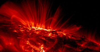
Some solar flares are associated with explosive coronal mass ejections, which can disturb Earth’s protective magnetosphere. The resulting geomagnetic storms generate dazzling auroras, but they can also interrupt radio communications and damage power grids. [SOHO (ESA & NASA)]

To Erupt or Not to Erupt

When a solar flare is blissfully unaccompanied by a violent eruption of plasma from the Sun’s surface, we call it a confined flare — the solar atmosphere remains bound to the surface rather than lashing out into interplanetary space. An eruptive flare, on the other hand, occurs when a coronal mass ejection is released along with the solar flare, exploding material out into the Sun’s surroundings.

It’s not yet clear why some solar flares are confined while others are eruptive. One possibility has to do with the arrangement of the Sun’s complex magnetic field. Twisted and tangled field lines can rearrange themselves through a process called magnetic reconnection, which accelerates charged particles and heats the plasma.

If, after reconnection, the magnetic field is either in a low-energy configuration or it’s sufficiently constricted by stronger magnetic fields farther from the Sun’s surface, no eruption will occur and the flare is confined. But how can we figure out what actually happens during confined flares?

Out on a Limb

The July 24, 2016, solar flare as seen in three extreme ultraviolet channels by Solar Dynamics Observatory. Panels a, b, and c show the progression of the flare from the beginning to the peak to the end. Click to enlarge. [Ning et al. 2018]

To better understand what makes solar flares tick, researchers often trace the movement of magnetic field loops before, during, and after the event. However, many flares are observed against the background of the bright solar disk, which can make it difficult to track the behavior of the magnetic loops.

To sidestep this issue, Hao Ning (Shandong University, China) and collaborators investigated the magnetic configuration of a flare extending from the edge of the Sun’s disk — the solar limb — where the bright arcs of plasma are clearly silhouetted against the dark background of the sky.

Ning and collaborators combined observations of a confined flare from the space-based observatories Solar Dynamics Observatory (SDO) and Ramaty High Energy Solar Spectroscopic Imager (RHESSI), as well as the Nobeyama Radioheliograph on the ground.

Time Evolution of a Solar Flare

Light curves extracted from the flaring region showed not one peak but two, which is thought to signal the presence of magnetic reconnection. Why two peaks? Magnetic reconnection in the corona accelerates charged particles, which then interact with the relatively dense chromospheric plasma. This interaction produces high-energy X-rays (the first peak) and heats the plasma, causing it to emit thermally at lower-energy X-ray wavelengths after a short delay (the second peak).

Soft X-ray light curves from RHESSI and hard X-ray light curves from the Geostationary Operational Environmental Satellite (GOES). The two peaks are labeled Stage A and B. The double-peaked behavior is evident at almost all energies. Click to enlarge. [Ning et al. 2018]

What makes this particular confined flare interesting is the range of wavelengths that exhibit the double peak — reaching energies as high as 50 keV (30 million K). This is a departure from previous observations of double-peaked flares, which have a lower-energy secondary peak.

Because of the unusually high energy, Ning and collaborators conclude that the plasma must be heated not only indirectly, by collisions with particles accelerated by reconnection, but also directly, by reconnection itself. This observation of a super-hot plasma component in the second stage of a confined flare is the first of its kind — and surely further observations will reveal new details of how confined flares evolve, continuing to build our picture of what determines confinement vs. eruption!

Citation

Hao Ning et al 2018 ApJ 854 178. doi:10.3847/1538-4357/aaaa69

27 June 2018

Peering Inside the Pillars of Creation

On 1 April 1995, Hubble captured one of its most well-known images: a stunning photo of towering features known as the Pillars of Creation, located in the Eagle Nebula just 7,000 light-years away. A new study explores how these iconic columns are influenced by the magnetic fields within them.

Pillars from Shocks

An illustrative figure of the BISTRO magnetic-field vectors observed in the Pillars of Creation, overlaid on a Hubble composite of the pillars. [Pattle et al. 2018]

In the Hubble image, we see the result of young, hot stars that have driven a photoionization shock into the cloud around them, forming complex structures in the dense gas at the shock interfaces. These structures — in this case, dense columns of neutral gas and dust — are then bombarded with hot radiation from the young stars, giving the structures a misty, ethereal look as they photoevaporate.

Though we have a rough picture, the specifics of how the Pillars of Creation were formed and how they evolve in this harsh radiation environment aren’t yet fully understood. In particular, the role of magnetic fields in shaping and sustaining these pillars is poorly constrained, both observationally and theoretically.

To address this problem, a team of scientists led by Kate Pattle (University of Central Lancashire, UK and National Tsing Hua University, Taiwan), has now made the first direct observations of the magnetic-field morphology within the Pillars of Creation.

The authors’ proposed formation scenario: a) an ionization front approaches an overdensity in the molecular gas, b) the front is slowed at the overdensity, causing the magnetic field lines to bend, c) the compressed magnetic field supports the pillar against radial collapse, but can’t support against longitudinal erosion. [Adapted from Pattle et al. 2018]

Observing Fields

Pattle and collaborators imaged the pillars as a part of the B-Fields in Star-Forming Region Observations (BISTRO) project, which uses a camera and polarimeter mounted on the James Clerk Maxwell Telescope in Hawaii. The high-resolution, submillimeter-wavelength polarimetric observations allowed the team to measure the orientations of the magnetic fields within the pillars.

Pattle and collaborators found that the magnetic fields inside the Pillars of Creation are actually quite organized: they generally run along the length of the pillars, perpendicular to and decoupled from the field in the surrounding cloud. The authors use their observations to estimate the strength of the fields: roughly 170–320 µG in the pillars.

Magnetic Support

What do these results tell us? First, the strength of the fields is consistent with a formation scenario in which very weakly magnetized gas was compressed to form columns. The authors propose that the Pillars of Creation were formed when an ionization front — driven by radiation from nearby young, hot stars — encountered a dense clump as it moved through the cloud of molecular gas. The overdensity slowed the front, causing the magnetic field to bend as the surrounding gas moved. The compressed magnetic field then supported the resulting column from collapse.

Pattle and collaborators argue that the magnetic fields in the Pillars of Creation are supporting the pillars radially against collapse even now. They may also be preventing the pillar ends from breaking off into disconnected clumps known as cometary globules, a process that could eventually disintegrate the pillars.

So what’s BISTRO up to now? The project is continuing to survey magnetic fields in the dense gas of other nearby high-mass star-forming regions. This may help confirm the results found for the Pillars of Creation, bringing us another step closer to understanding how magnetic fields influence the some of the striking features that Hubble and other telescopes have revealed in our astronomical backyard.

Citation

Kate Pattle et al 2018 ApJL 860 L6. doi:10.3847/2041-8213/aac771

22 June 2018

Identifying Life from Varying Atmospheres

There’s no hiding — changes in Earth’s atmosphere over the seasons are a dead giveaway to the fact that Earth hosts life. Now a new study explores whether we might use atmospheric seasonality like Earth’s to detect life on other planets.

Looking for Change

Most of the searches for life beyond our planet focus on identifying static biosignatures, like the presence of methane or large amounts of oxygen in an exoplanetary atmosphere. This approach suffers from many ambiguities, however — including a high likelihood of false positives (processes that chemically mimic life signatures but aren’t life) and false negatives (non-detections despite the presence of life).

Earth’s atmospheric carbon dioxide (top) and methane (bottom) levels vary seasonally, as seen in these data from NOAA’s Earth System Research Laboratory. [Olson et al. 2018]

In a new study led by Stephanie Olson (UC Riverside and NASA Astrobiology Institute Alternative Earths and Virtual Planetary Laboratory Teams), a team of scientists has proposed an alternative approach: to search for distinctive variability of exoplanet atmospheres that indicates the presence of life.

Seasons and Life

if you’re like me, you probably haven’t spent a lot of time thinking about interactions between the Earth’s biosphere and its axial tilt. Nonetheless, this interplay is responsible for detectable and distinctive seasonal changes in our planet’s atmosphere!

This schematic shows how oxygen and carbon dioxide levels in the atmosphere vary in opposing phase seasonally, with the increased sunlight in summer driving greater conversion of carbon dioxide into oxygen. [Olson et al. 2018]

Since so much of our globe is covered by photosynthesizing life, the seasonal availability of sunlight regulates the conversion of carbon dioxide to oxygen, providing a signature in our atmosphere that varies over the course of the year. And photosynthesis isn’t the only culprit! Other biological products evolve seasonally as well — as the surface temperature on our globe changes throughout the year, biological rates, gas solubility, precipitation patterns, and more all respond accordingly.

Olson and collaborators ask a simple question: if our atmosphere varies distinctively in a way that reveals the presence of life on Earth, can we search for similar variation on other planets?

Gaseous Signatures

To answer this question, Olson and collaborators examine the potential for seasonal variation of several atmospheric gases: carbon dioxide, methane, molecular oxygen, and ozone. For a weakly oxygenated planet (like early Earth), the authors find that a detectable indicator of life may be seasonal variations in the strength of ozone spectral bands at ultraviolet wavelengths. This variation serves as a tracer of the seasonality of molecular oxygen.

On a planet with the right conditions, seasonal oxygen oscillations could create an observable difference in the depth of the ozone spectral line, as shown here. [Adapted from Olson et al. 2018]

To discover such a signature in the atmospheres of distant planets, we’ll likely need extended direct imaging; transit spectroscopy, such as that expected from the James Webb Space Telescope, will probe planets at only one point in their orbits, precluding the detection of seasonal changes. Olson and collaborators therefore advocate that upcoming direct-imaging missions, like LUVOIR and HabEx, include ultraviolet observing capabilities.

What is the likelihood that we’ll actually be able to detect seasonal changes in the atmospheric gases of distant exoplanets? More detailed modeling will need to be performed to say for certain — but in the meantime, this study presents an interesting additional technique we can add to our arsenal and explore further in the future!

Citation

Stephanie L. Olson et al 2018 ApJL 858 L14. doi:10.3847/2041-8213/aac171

20 June 2018

Exploring Jets from a Supermassive Black Hole

What are the feeding — and burping — habits of the supermassive black holes peppering the universe? In a new study, observations of one such monster reveal more about the behavior of its powerful jets.

Beams from Behemoths

Across the universe, supermassive black holes of millions to billions of solar masses lie at the centers of galaxies, gobbling up surrounding material. But not all of the gas and dust that spirals in toward a black hole is ultimately swallowed! A large fraction of it can instead be flung out into space again, in the form of enormous, powerful jets that extend for thousands or even millions of light-years in opposite directions.

M87, shown in this Hubble image, is a classic example of a nearby (55 million light-years distant) supermassive black hole with a visible, collimated jet. Its counter-jet isn’t seen because relativistic effects make the receding jet appear less bright. [The Hubble Heritage Team (STScI/AURA) and NASA/ESA]

What causes these outflows to be tightly beamed — collimated — in the form of jets, rather than sprayed out in all directions? Does the pressure of the ambient medium — the surrounding gas and dust that the jet is injected into — play an important role? In what regions do these jets accelerate and decelerate? There are many open questions that scientists hope to understand by studying some of the active black holes with jets that live closest to us.

Eyes on a Nearby Giant

In a new study led by Satomi Nakahara (The Graduate University for Advanced Studies in Japan), a team of scientists has used multifrequency Very Long Baseline Array (VLBA) and Very Long Array (VLA) images to explore jets emitted from a galaxy just 100 million light-years away: NGC 4261.

This galaxy’s (relatively) close distance — as well as the fact that we’re viewing it largely from the side, so we can clearly see both of its polar jets — allows us to observe in detail the structure and intensity of its jets as a function of their distance from the black hole. Nakahara and collaborators’ observations span the enormous radial distance of a thousand to a billion times the radius of the black hole, or about 54 light-days to more than a million light-years.

Scale for Change

The width of the jet as a function of radial distance from the black hole, for NGC 4261 (red) compared to the few other jets from nearby supermassive black holes that we’ve measured. NGC 4261’s jets transition from parabolic to conical at around 10,000 times the radius of the black hole (R_S). [Nakahara et al. 2018]

The authors’ observations of NGC 4261’s jets indicate that a transition occurs at ~10,000 times the radius of the black hole (that’s a little over a light-year from the black hole). At this point, the jets’ structures change from parabolic (becoming more tightly beamed) to conical (expanding freely). Around the same location, Nakahara and collaborators also see the radiation profile of one of the jets change, suggesting the physical conditions in the jets transition here as well.

This is the first time we’ve been able to examine jet width this closely for both of the jets emitted from a supermassive black hole. The fact that the structure changes at the same distance for both jets indicates that the shape of these powerful streams is likely governed by global properties of the environment surrounding the galaxy’s nucleus, or properties of the jets themselves, rather than by a local condition.

The authors next hope to pin down velocities inside NGC 4261’s jets to determine where the jets accelerate and decelerate. This nearby powerhouse is clearly going to be a useful laboratory in the future, helping to unveil the secrets of more distant, feeding monsters.

Bonus

Curious what these hungry supermassive black holes look like? Check out this artist’s imagining of NGC 4261, which shows how it feeds from a large, swirling accretion disk and emits fast-moving, collimated jets. [Original video credit to Dana Berry, Space Telescope Science Institute]

Citation

Satomi Nakahara et al 2018 ApJ 854 148. doi:10.3847/1538-4357/aaa45e

18 June 2018

Using Satellite Galaxies to Weigh the Milky Way

Weighing galaxies is a tricky business — especially when that galaxy is our own! In a recent study, scientists have tackled this problem by harnessing incredibly precise measurements of the motions of Milky-Way satellites.

A Challenging Measurement

Locations of some of the ~50 satellite galaxies known around the Milky Way. [AndrewRT]

Our spot in the middle of our galaxy’s disk makes it difficult for us to assess the total mass of gas, dust, stars, and dark matter surrounding us; estimates for the Milky Way’s mass span from 700 billion to 2 trillion solar masses! Pinning down this number is critical for better understanding the structure and dynamics of our local universe.

So what’s the key to precisely weighing the Milky Way? A new study led by Ekta Patel (University of Arizona) — presented at the American Astronomical Society meeting two weeks ago — suggests it may be the barely preceptible motions of the small satellite galaxies that orbit around the Milky Way. Around 50 Milky-Way satellites are currently known, and simulations suggest that there may be up to 100–200 in total. By watching the motions of these satellites, we can trace the potential of their host — the Milky Way — and estimate its mass.

The Illustris-Dark simulation evolves our universe to the present day, providing a view of how dark matter organizes itself into galaxy halos over time. [Illustris Collaboration]

Tiny Motions of Tiny Galaxies

In this era of precision astronomy, remarkable measurements are becoming possible. In their study, Patel and collaborators use years of proper-motion observations from the Hubble Space Telescope for nine satellite galaxies of the Milky Way. The precision needed for measurements like these is insane: watching these satellites move is roughly like watching a human hair grow at the distance of the Moon.

Rather than using the instantaneous position and velocity measured for a satellite — which changes over time during the satellite’s orbit — Patel and collaborators demonstrate that the satellite’s specific angular momentum is a more useful parameter when attempting to estimate its host galaxy’s mass.

For each of the nine individual satellite galaxies, the authors compare its measured momentum to that of ~90,000 simulated satellite galaxies from the Illustris-Dark cosmological simulation. This matching is used to build a probability distribution for the mass of the host galaxy most likely to be orbited by such a satellite. The probability distributions for the nine satellite galaxies are then combined to find the best overall estimate for the Milky Way’s mass.

Tipping the Scale

Top: summary of the most likely Milky-Way mass estimated from each of the 9 satellite galaxies, using the instantaneous positions and velocities (left) and the momentum (right) of the satellites. The momentum method shows less scatter in the host masses. Bottom: probability distributions for the most likely Milky-Way mass for each of the satellites (colored curves) and combined (grey curve). Click for a better look. [Patel et al. 2018]

Using this technique, Patel and collaborators find a mass of 0.96 trillion solar masses for the Milky Way. The error bars for their measurement are around 30% — and while this is more confined than the broad range of past estimates, it’s not yet extremely precise. The beauty of Patel and collaborators’ method, however, is that it is both extendable and generalizable.

The authors only had access to precise proper motions for nine satellite galaxies when they conducted their study — but since then, the Gaia mission has provided measurements for 30 satellites, with more expected in the future. Including these additional satellites and using improved, higher-resolution cosmological simulations for comparison will continue to increase the precision of Patel and collaborators’ estimate in the future.

In addition, this approach can also be used to weigh our neighboring Andromeda galaxy, or any other galaxy for which we’re able to get precise proper-motion measurements for its satellites. Keep an eye out in the future, as techniques like this continue to reveal more properties of our local universe.

Citation

Ekta Patel et al 2018 ApJ 857 78. doi:10.3847/1538-4357/aab78f

15 June 2018

Stellar by Day, Planetary by Night: Atmospheres of Ultra-Hot Jupiters

Move over, hot Jupiters — there’s an even stranger kind of giant planet in the universe! Ultra-hot Jupiters are so strongly irradiated that the molecules in their atmospheres split apart. What does this mean for heat transport on these planets?

Atmospheres of Exotic Planets

A diagram showing the orbit of an ultra-hot Jupiter and the longitudes at which dissociation and recombination occur. [Bell & Cowan 2018]

Similar to hot Jupiters, ultra-hot Jupiters are gas giants with atmospheres dominated by molecular hydrogen. What makes them interesting is that their dayside atmospheres are so hot that the molecules dissociate into individual hydrogen atoms — more like the atmospheres of stars than planets.

Because of the intense stellar irradiation, there is also an extreme temperature difference between the day and night sides of these planets — potentially more than 1,000 K! As the stellar irradiation increases, the dayside atmosphere becomes hotter and hotter and the temperature difference between the day and night sides increases.

When hot atomic hydrogen is transported into cooler regions (by winds, for instance), it recombines to form H₂ molecules and heats the gas, effectively transporting heat from one location to another. This is similar to how the condensation of water redistributes heat in Earth’s atmosphere — but what effect does this phenomenon have on the atmospheres of ultra-hot Jupiters?

Maps of atmospheric temperature of molecular hydrogen dissociation fraction for three wind speeds. Click to enlarge. [Bell & Cowan 2018]

Modeling Heat Redistribution

Taylor Bell and Nicolas Cowan (McGill University) used an energy-balance model to estimate the effects of H₂ dissociation and recombination on heat transport in ultra-hot Jupiter atmospheres. In particular, they explored the redistribution of heat and how it affects the resultant phase curve — the curve that describes the combination of reflected and thermally emitted light from the planet, observed as a function of its phase angle.

For reasonable eastward wind speeds, Bell and Cowan found that the recombination of atomic hydrogen shifts the peak of the phase curve in the eastward direction, with the shift becoming more pronounced with increasing eastward wind speed. Additionally, because heat is distributed more evenly across the planet, including this process decreases the amplitude of the phase variations.

A Bright Future for Ultra-hot Jupiters

Theoretical phase curves for three wind speeds. Transits and eclipses have been neglected. [Bell & Cowan 2018]

While this simple model doesn’t include potentially important effects such as the changing atmospheric opacity as a function of longitude or formation of clouds on the planet’s nightside, this result indicates that caution is required when interpreting phase curves of ultra-hot Jupiters. For example, neglecting recombination means assuming a lower heat transport efficiency, which will require artifically high wind speeds to match observed phase curves.

Only a few ultra-hot Jupiters are currently known, but that will soon change. The Transiting Exoplanet Survey Satellite (TESS) mission, which is set to begin its first science observations on June 17, 2018, will search for exoplanets around bright stars, including nearby cool stars and more distant hot stars. The hot stars may play host to these exotic exoplanets, and upcoming observations of ultra-hot Jupiters like KELT-9b will put this theory of heat redistribution to the test.

Citation

Taylor J. Bell & Nicolas B. Cowan 2018 ApJL 857 L20. doi:10.3847/2041-8213/aabcc8

Previous 1 … 86 87 88 89 90 … 122 Next