Features Archives - Page 82 of 112

Features RSS

9 March 2018

Signs of Asymmetry in Exploding Stars

Supernova explosions enrich the interstellar medium and can even briefly outshine their host galaxies. However, the mechanism behind these massive explosions still isn’t fully understood. Could probing the asymmetry of supernova remnants help us better understand what drives these explosions?

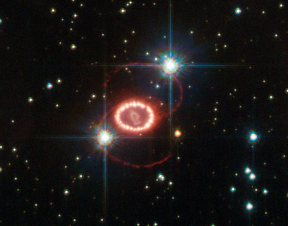
Hubble image of the remnant of supernova 1987A, one of the first remnants discovered to be asymmetrical. [ESA/Hubble, NASA]

Stellar Send-Offs

High-mass stars end their lives spectacularly. Each supernova explosion churns the interstellar medium and unleashes high-energy radiation and swarms of neutrinos. Supernovae also suffuse the surrounding interstellar medium with heavy elements that are incorporated into later generations of stars and the planets that form around them.

The bubbles of expanding gas these explosions leave behind often appear roughly spherical, but mounting evidence suggests that many supernova remnants are asymmetrical. While asymmetry in supernova remnants can arise when the expanding material plows into the non-uniform interstellar medium, it can also be an intrinsic feature of the explosion itself.

Simulation results clockwise from top left: Mass density, calcium mass fraction, oxygen mass fraction, nickel-56 mass fraction. Click to enlarge. [Adapted from Wollaeger et al. 2017]

Coding Explosions

The presence — or absence — of asymmetry in a supernova remnant can hold clues as to what drove the explosion. But how can we best observe asymmetry in a supernova remnant? Modeling lets us explore different observational approaches.

A team of scientists led by Ryan T. Wollaeger (Los Alamos National Laboratory) used radiative transfer and radiative hydrodynamics simulations to model the explosion of a core-collapse supernova. Wollaeger and collaborators introduced asymmetry into the explosion by creating a single-lobed, fast-moving outflow along one axis.

Their simulations showed that while some chemical elements lingered near the origin of the explosion or were distributed evenly throughout the remnant, calcium was isolated to the asymmetrical region, hinting that spectral lines of calcium may be good tracers of asymmetry.

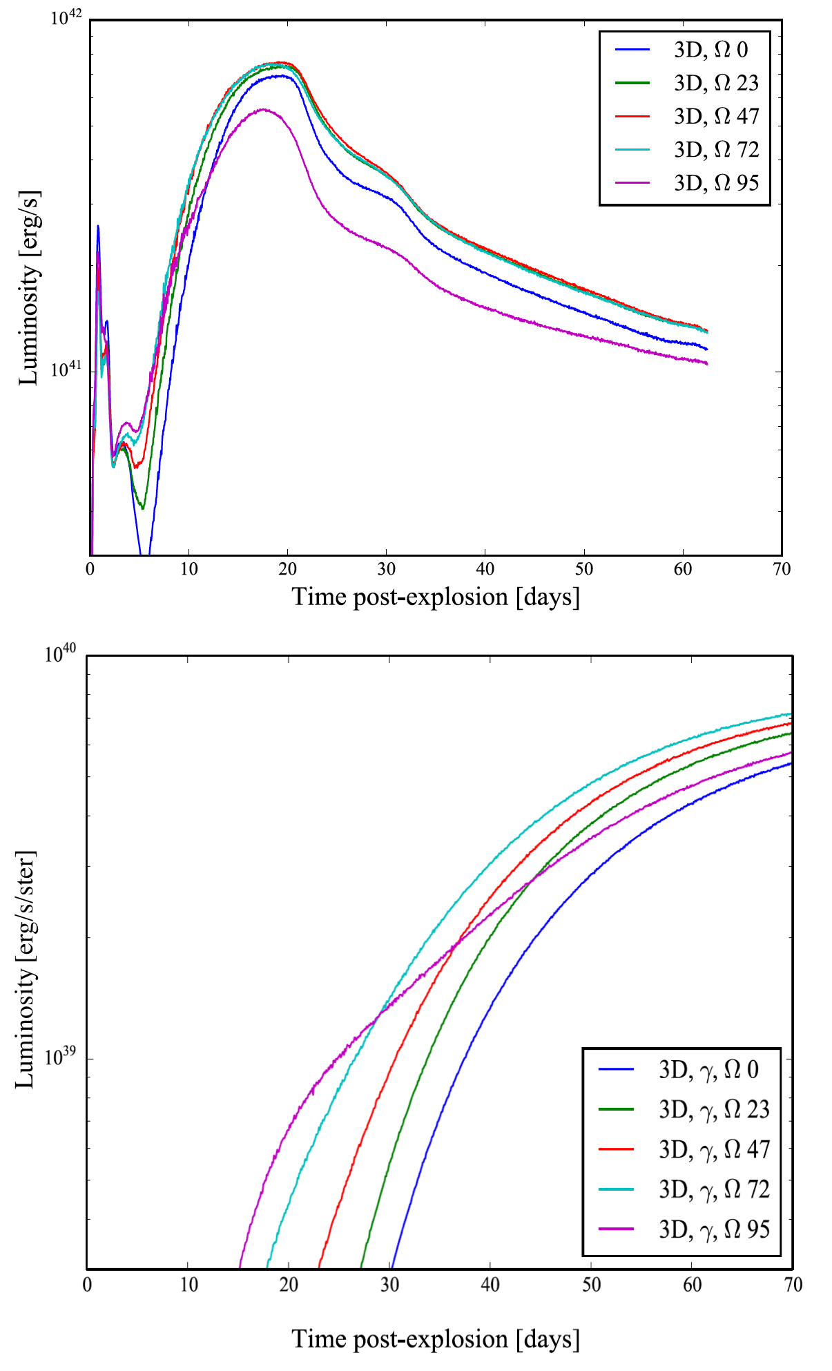
Bolometric (top) and gamma-ray (bottom) synthetic light curves for the authors’ model for a range of simulated viewing angles. [Adapted from Wollaeger et al. 2017]

Synthesizing Spectra

Wollaeger and collaborators then generated synthetic light curves and spectra from their models to determine which spectral features or characteristics indicated the presence of the asymmetric outflow lobe. They found that when an asymmetric outflow lobe is present, the peak luminosity of the explosion depends on the angle at which you view it; the highest luminosity occurs when the lobe is viewed from the side, while the lowest luminosity — nearly 40% dimmer — is seen when the explosion is viewed “down the barrel” of the lobe. The dense outflow shades the central radioactive source from view, lowering the luminosity.

This effect also plays out in the gamma-ray light curves; when viewed down the barrel, the shading of the central source by a high-density lobe slows the rise of the gamma-ray luminosity and changes the shape of the light curve compared to views from other vantage points.

Another promising avenue for exploring asymmetry is a near-infrared band encompassing an emission line of singly-ionized calcium near 815 nm. Since calcium is confined within the outflow lobe in the simulation, its emission lines are blueshifted when the lobe points toward the observer.

The authors point out that there is much more to be done in their models, such as including the effects of shock heating of circumstellar material, which can contribute strongly to the light curve, but these simulations bring us a step closer to understanding the nature of asymmetrical supernova remnants — and the explosions that create them.

Citation

Ryan T. Wollaeger et al 2017 ApJ 845 168. doi:10.3847/1538-4357/aa82bd

7 March 2018

The Fate of Exomoons when Planets Scatter

Four examples of close-encounter outcomes: a) the moon stays in orbit around its host, b) the moon is captured into orbit around its perturber, c) and d) the moon is ejected from the system from two different starting configurations. [Adapted from Hong et al. 2018]

Planet interactions are thought to be common as solar systems are first forming and settling down. A new study suggests that these close encounters could have a significant impact on the moons of giant exoplanets — and they may generate a large population of free-floating exomoons.

Chaos in the System

In the planet–planet scattering model of solar-system formation, planets are thought to initially form in closely packed systems. Over time, planets in a system perturb each other, eventually entering an instability phase during which their orbits cross and the planets experience close encounters.

During this “scattering” process, any exomoons that are orbiting giant planets can be knocked into unstable orbits directly by close encounters with perturbing planets. Exomoons can also be disturbed if their host planets’ properties or orbits change as a consequence of scattering.

Led by Yu-Cian Hong (Cornell University), a team of scientists has now explored the fate of exomoons in planet–planet scattering situations using a suite of N-body numerical simulations.

Chances for Survival

Hong and collaborators find that the vast majority — roughly 80 to 90% — of exomoons around giant planets are destabilized during scattering and don’t survive in their original place in the solar system. Fates of these destabilized exomoons include:

moon collision with the star or a planet,
moon capture by the perturbing planet,
moon ejection from the solar system,
ejection of the entire planet–moon system from the solar system, and
moon perturbation onto a new heliocentric orbit as a “planet”.

Unsurprisingly, exomoons that have close-in orbits and those that orbit larger planets are the most likely to survive close encounters; as an example, exomoons on orbits similar to Jupiter’s Galilean satellites (i.e., orbiting at a distance of less than 4% of their host planet’s Hill radius) have a ~20–40% chance of survival.

Moon initial semimajor axis vs. moon survival rate. Three of Jupiter’s Galilean moons are shown for reference. [Hong et al. 2018]

Free-Floating Moons

An intriguing consequence of Hong and collaborators’ results is the prediction of a population of free-floating exomoons that were ejected from solar systems during planet–planet scattering and now wander through the universe alone. According to the authors’ models, there may be as many of these free-floating exomoons as there are stars in the universe!

Future surveys that search for objects using gravitational microlensing — like that planned with the Wide-Field Infrared Survey Telescope (WFIRST) — may be able to detect such objects down to masses of a tenth of an Earth mass. In the meantime, we’re a little closer to understanding the complex dynamics of early solar systems.

Citation

Yu-Cian Hong et al 2018 ApJ 852 85. doi:10.3847/1538-4357/aaa0db

28 February 2018

Jets from Young Stars in Cygnus-X

How do you spot very young, newly formed stars? One giveaway is the presence of jets and outflows that interact with the stars’ environments. In a new study, scientists have now discovered an unprecedented number of these outflows in a nearby star-forming region of our galaxy.

Young Stars Hard at Work

CO map of the Cygnus-X region of the galactic plane, with the grid showing the UWISH2 coverage and the black triangles showing the positions of the detected outflows. [Makin & Froebrich 2018]

The birth and evolution of young stars is a dynamic, energetic process. As new stars form, material falls inward from the accretion disks surrounding young stellar objects, or YSOs. This material can power collimated streams of gas and dust that flow out along the stars’ rotation axes, plowing through the surrounding material. Where the outflows collide with the outside environment, shocks form that can be spotted in near-infrared hydrogen emission.

Though we’ve learned a lot about these outflows, there remain a number of open questions. What factors govern their properties, such as their lengths, luminosities, and orientations? What is the origin of the emission features we see within the jets, known as knots? What roles do the driving sources and the environments play in the behavior and appearance of the jets?

A selection of previously unknown outflows discovered as a result of this survey. Click for a closer look. [Makin & Froebrich 2018]

To answer these questions, we need to build a large, unbiased statistical sample of YSOs from across the galactic plane. Now, a large infrared survey — known as the UKIRT Widefield Infrared Survey for H₂ (UWISH2) — is working toward that goal.

Jackpot in Cygnus-X

In a recent publication, Sally Makin and Dirk Froebrich (University of Kent, UK), present results from UWISH2’s latest release: a survey segment targeting a 42-square-degree region in the galactic plane known as the Cygnus-X star-forming region.

The team’s search for shock-excited emission in Cygnus-X yielded spectacular results. They found a treasure trove of outflows — a remarkable 572 in total, representing a huge increase over the 107 known previously.

Makin and Froebrich then measured properties of the outflows themselves — such as length, orientation, and flux — as well as properties of the sources that appear to drive them.

Pinning Down Properties

This low-mass bright-rimmed cloud near IRAS 20294+4255 contains a number of stellar outflows. It may warrant further study as a classical example of triggered star formation. [Makin & Froebrich 2018]

Of the 572 outflows, the authors found that 27% are one-sided jets and 46% are bipolar. The bipolar outflows are typically ~1.5 light-years in total length, and they are frequently asymmetric, with the shorter jet lobe averaging only 70% the length of the longer one. The flux from the two sides of bipolar jets is also often asymmetric: typically one side is brighter by about 50%.

Exploring the knots of bright emission within the outflows, the authors found that they are typically closely spaced, suggesting that the material generating them is ejected every 900–1,400 years. This rapid production — faster than what has been found in YSO outflows in other regions — rules out some models of how these knots are produced.

Based on the fraction of UWISH2 data analyzed so far, the authors estimate that the entire UWISH2 survey will uncover a total of ~2,000 jets and outflows from YSOs. This large, unbiased new sample is finally allowing astronomers to build out the statistics of YSO outflows to better understand them.

Citation

S. V. Makin and D. Froebrich 2018 ApJS 234 8. doi:10.3847/1538-4365/aa8862

26 February 2018

PALFA Discovers Neutron Stars on a Collision Course

Got any plans in 46 million years? If not, you should keep an eye out for PSR J1946+2052 around that time — this upcoming merger of two neutron stars promises to be an exciting show!

Survey Success

Average profile for PSR J1946+2052 at 1.43 GHz from a 2 hr observation from the Arecibo Observatory. [Stovall et al. 2018]

It seems like we just wrote about the dearth of known double-neutron-star systems, and about how new surveys are doing their best to find more of these compact binaries. Observing these systems improves our knowledge of how pairs of evolved stars behave before they eventually spiral in, merge, and emit gravitational waves that detectors like the Laser Interferometer Gravitational-wave Observatory might observe.

Today’s study, led by Kevin Stovall (National Radio Astronomy Observatory), goes to show that these surveys are doing a great job so far! Yet another double-neutron-star binary, PSR J1946+2052, has now been discovered as part of the Arecibo L-Band Feed Array pulsar (PALFA) survey. This one is especially unique due to the incredible speed with which these neutron stars orbit each other and their correspondingly (relatively!) short timescale for merger.

An Extreme Example

The PALFA survey, conducted with the enormous 305-meter radio dish at Arecibo, has thus far resulted in the discovery of 180 pulsars — including two double-neutron-star systems. The most recent discovery by Stovall and collaborators brings that number up to three, for a grand total of 16 binary-neutron-star systems (confirmed and unconfirmed) known to date.

The 305-m Arecibo Radio Telescope, built into the landscape at Arecibo, Puerto Rico. [NOAO/AURA/NSF/H. Schweiker/WIYN]

The newest binary in this collection, PSR J1946+2052, exhibits a pulsar with a 17-millisecond spin period that whips around its compact companion at a terrifying rate: the binary period is just 1.88 hours. Follow-up observations with the Jansky Very Large Array and other telescopes allowed the team to identify the binary’s location to high precision and establish additional parameters of the system.

PSR J1946+2052 is a system of extremes. The binary’s total mass is found to be ~2.5 solar masses, placing it among the lightest binary-neutron-star systems known. Its orbital period is the shortest we’ve observed, and the two neutron stars are on track to merge in less time than any other known neutron-star binaries: in just 46 million years. When the two stars reach the final stages of their merger, the effects of the pulsar’s rapid spin on the gravitational-wave signal will be the largest of any such system discovered to date.

More Tests of General Relativity

What can PSR J1946+2052 do for us? This extreme system will be especially useful as a gravitational laboratory. Continued observations of PSR J1946+2052 will pin down with unprecedented precision parameters like the Einstein delay and the rate of decay of the binary’s orbit due to the emission of gravitational waves, testing the predictions of general relativity to an order of magnitude higher precision than was possible before.

As we expect there to be thousands of systems like PSR J1946+2052 in our galaxy alone, better understanding this binary — and finding more like it — continue to be important steps toward interpreting compact-object merger observations in the future.

Citation

K. Stovall et al 2018 ApJL 854 L22. doi:10.3847/2041-8213/aaad06

23 February 2018

Our Galactic Neighbor Hosts Complex Organic Molecules

For the first time, data from the Atacama Large Millimeter/submillimeter Array (ALMA) reveal the presence of methyl formate and dimethyl ether in a star-forming region outside our galaxy. This discovery has important implications for the formation and survival of complex organic compounds — important for the formation of life — in low-metallicity galaxies both young and old.

No Simple Picture of Complex Molecule Formation

ALMA, pictured here with the Magellanic Clouds above, has observed organic molecules in our Milky Way Galaxy —
and beyond. [ESO/C. Malin]

Complex organic molecules (those with at least six atoms, one or more of which must be carbon) are the precursors to the building blocks of life. Knowing how and where complex organic molecules can form is a key part of understanding how life came to be on Earth — and how it might arise elsewhere in the universe. From exoplanet atmospheres to interstellar space, complex organic molecules are ubiquitous in the Milky Way.

In our galaxy, complex organic molecules are often found in the intense environments of hot cores — clumps of dense molecular gas surrounding the sites of star formation. However, it’s not yet fully understood how the complex organic molecules found in hot cores come to be. One possibility is that the compounds condense onto cold dust grains long before the young stars begin heating their natal shrouds. Alternatively, they might assemble themselves from the hot, dense gas surrounding the blazing protostars.

Composite infrared and optical image of the N 113 star-forming region in the LMC. The ALMA coverage is indicated by the gray line. Click to enlarge. [Sewiło et al. 2018]

Detecting Complexity, a Galaxy Away

Using ALMA, a team of researchers led by Marta Sewiło (NASA Goddard Space Flight Center) recently detected two complex organic molecules — methyl formate and dimethyl ether — for the first time in our neighboring galaxy, the Large Magellanic Cloud (LMC). Previous searches for organic molecules in the LMC detected small amounts of methanol, the parent molecule of the two newly-discovered compounds. By revealing the spectral signatures of dimethyl ether and methyl formate, Sewiło and collaborators further prove that organic chemistry is hard at work in hot cores in the LMC.

This discovery is momentous because dwarf galaxies like the LMC tend to have a lower abundance of the heavy elements that make up complex organic molecules — most importantly, oxygen, carbon, and nitrogen. Beyond lacking the raw materials necessary to create complex molecules, the gas of low-metallicity galaxies does a poorer job preventing the penetration of high-energy photons. The impinging photons warm dust grains, resulting in a lower probability of forming and maintaining complex organic molecules. Despite this, organic molecules appear to be able to develop and persist — which has exciting implications for organic chemistry in low-metallicity environments.

ALMA observation of emission by methyl formate in a hot core in the LMC.
[Adapted from Sewiło et al. 2018]

A Lens into the Past

In the early universe, before the budding galaxies have had time to upcycle their abundant hydrogen into heavier elements, organic chemistry is thought to proceed slowly or not at all. The discovery of complex organic molecules in a nearby low-metallicity galaxy upends this theory and propels us toward a better understanding of the organic chemistry in the early universe.

Citation

Marta Sewiło et al 2018 ApJL 853 L19. doi:10.3847/2041-8213/aaa079

21 February 2018

Driving Jets from the Sun

Could coronal mass ejections (bottom panel) be driven by the same mechanism as the much smaller coronal jets (top panel)? [NASA]

What launches small jets and enormous coronal mass ejections (CMEs) from the Sun’s surface? New simulations explore how changing magnetic fields can drive these powerful eruptions.

Different Sizes, Same Jets?

Coronal jets are frequent, short-lived eruptions of plasma that are launched from low in the Sun’s atmosphere and travel outward through the corona. These ejections occur frequently across the Sun’s surface, lasting for ~10 minutes at a time and reaching lengths of ~50,000 km — a few times the Earth’s diameter, but still tiny compared to their enormous cousins, CMEs.

Despite the difference in size scales, a team of scientists led by Peter Wyper of Durham University has proposed that both coronal jets and CMEs are launched by the same mechanism, a process known as “magnetic breakout”. In a recent publication, Wyper and collaborators show the results of a series of 3D magnetohydrodynamic simulations of coronal jets to see what we would expect to observe from magnetic-breakout-driven eruptions.

Breaking Free

In the magnetic breakout model, magnetic field lines above filaments break and reconnect, removing confinement and allowing the filament to erupt from the Sun’s surface. Wyper and collaborators simulate this process by modeling a small bipolar structure on the Sun’s surface, embedded in a background magnetic field. They then observe how the magnetic fields rearrange themselves over time.

Schematic of the evolutionary sequence that produces breakout jets. The growing, twisted flux rope is shown by the yellow field lines. [Wyper et al. 2017]

The coronal jets that form in these simulations have four main stages:

Filament channel formation
Free energy is stored in a mini-filament or flux rope embedded within a background larger-scale magnetic field.
Breakout
Slow reconnection of the magnetic field lines above the growing flux rope eventually leads to a critical point where the flux rope can rapidly reconnect with the external field, breaking out.
Eruptive jet
As the filament escapes, it rapidly unwinds its twist and accelerates surrounding plasma along with it, causing the sudden eruption of an energetic, helical jet.
Relaxation
After several minutes, the jet propagates away, the reconnection subsides, and the fields relax into a new equilibrium similar to the starting point.

A Match to Observations

Wyper and collaborators run three sets of simulations with differing inclinations of the background magnetic fields, and they show that magnetic breakout in all three cases can lead to the production of broad, twisting jets with features consistent with what we’ve observed on the Sun.

In particular, the differing background field inclinations lead to a diversity of reconnection outflows preceding the jets. For highly inclined fields, for instance, a fast, dense outflow is driven with an inverted Y shape; for vertical fields, the outflows form much weaker spires.

All of these behaviors have been observed, and Wyper and collaborators’ model ties them together into a unified picture of coronal jet launching that has also been proposed to describe CMEs on a larger scale. If this picture is correct, then it may be possible that the complexities of these different solar eruptions can all be boiled down to one underlying process.

Eruption sequence for an inclined background field at a) 16 minutes, b) 24 minutes, and c) 31 minutes. [Wyper et al. 2018]

Citation

P. F. Wyper et al 2018 ApJ 852 98. doi:10.3847/1538-4357/aa9ffc

16 February 2018

An Eccentric Planet Skims a Giant Star

As part of a major survey of evolved stars, scientists have discovered the most eccentric planet known to orbit a giant. What can we learn from this unusual object before it’s eventually consumed by its host?

Planetary Diversity

An example of the diversity of just a few of the planetary systems discovered by the Kepler mission. [NASA]

In the early stages of exoplanet science, it was easy to assume that all systems around other stars would be similar to our own solar system: rocky worlds close in, gas giants further out — and all with co-planar, low-eccentricity orbits.

As we observed the first exoplanets and learned about their properties, however, it quickly became apparent that most other systems don’t resemble our own. The more exoplanets we observe, the more we become aware of the diversity of planetary systems — with planet compositions, masses, and orbits unlike any in the solar system.

Orbit of HD 76920b, oriented properly and overlaid with the solar system inner planets’ orbits to scale. A comet and asteroid from our solar system are shown as having comparably eccentric orbits. [Wittenmyer et al. 2017]

Relative Sizes Matter

Some systems are easier to study than others. Since exoplanet detection and characterization techniques rely on looking for the imprint of planets on stellar signals, systems consisting of a small star and large planet are favored. For this reason, exoplanets orbiting solar-like or dwarf stars are especially well studied — but we don’t have nearly as much information about planets orbiting massive, hot stars.

To combat this lack of data, several teams have begun surveys particularly targeting evolved, massive stars. One of these is known as the Pan-Pacific Planet Search, a survey that uses the 3.9m Anglo-Australian Telescope in Australia to study the spectra of metal-rich subgiants in the southern hemisphere. Fresh among the discoveries from this survey is a planet orbiting HD 76920, reported on in a recent publication led by Robert Wittenmyer (University of Southern Queensland and University of New South Wales, Australia).

An Extreme Orbit

Orbital eccentricity vs. planet’s periastron distance for the 116 confirmed planets orbiting giant stars. HD 76920b, the most eccentric of them, is shown with the red dot. [Wittenmyer et al. 2017]

Wittenmyer and collaborators conducted follow-up spectroscopy with two additional telescopes to confirm the properties of HD 76920. The team reports that HD 76920b — a giant planet of perhaps 4 Jupiter masses, with a period of 415 days and an eccentricity of e = 0.86 — is the most eccentric planet ever discovered orbiting a giant star.

How did HD 76920b achieve its extreme orbit? The go-to explanation for such an orbit is gravitational influence from a distant, massive stellar companion — and yet the authors find no evidence in their observations for a second star in the system. Instead, the team suggests that HD 76020b arrived on its current orbit via planet–planet scattering interactions earlier in the system’s lifetime.

Artist’s impression of a planet being engulfed by its host star. [NASA/ESA/G. Bacon]

Toasty Future

Lastly, Wittenmyer and collaborators use modeling to explore HD 76020b’s future. This planet’s orbit is already so extreme that it nearly skims the surface of its host, dipping to within 4 stellar radii of the star’s surface at its closest approach. The authors show that the planet will be engulfed by its host on a timescale of ~100 million years due to a combination of the star’s expanding radius and tidal interactions.

Gathering more observations of this extreme planet — and hunting for others like it — will help us to continue to learn about the formation and evolution of the diverse planetary systems our universe houses.

Citation

Robert A. Wittenmyer et al 2017 AJ 154 274. doi:10.3847/1538-3881/aa9894

14 February 2018

Galactic Pairs in the Early Universe

In the spirit of Valentine’s Day, today we’ll be exploring apparent pairs of galaxies in the distant, early universe. How can we tell whether these duos are actually paired galaxies, as opposed to disguised singles?

Real Pair, or Trick of the Light?

In the schematic timeline of the universe, the epoch of reionization is when the first galaxies and quasars began to form and evolve. [NASA]

The statistics of merging galaxies throughout the universe reveal not only direct information about how galaxies interact, but also cosmological information about the structure of the universe. While we’ve observed many merging galaxy pairs at low redshift, however, it’s much more challenging to identify these duos in the early universe.

A merging pair of galaxies at high redshift appears to us as a pair of unresolved blobs that lie close to each other in the sky. But spotting such a set of objects doesn’t necessarily mean we’re looking at a merger! There are three possible scenarios to explain an observed apparent duo:

It’s a pair of galaxies in a stage of merger.
It’s a projection coincidence; the two galaxies aren’t truly near each other.
It’s a single galaxy being gravitationally lensed by a foreground object. This strong lensing produces the appearance of multiple galaxies.

Hubble photometry of one of the three galaxy groups identified at z ~ 8, with the galaxies in the image labeled with their corresponding approximate photometric redshifts. [Adapted from Chaikin et al. 2018]

Hunting for Distant Duos

In a recent study led by Evgenii Chaikin (Peter the Great St. Petersburg Polytechnic University, Russia), a team of scientists has explored the Hubble Ultra Deep Field in search of high-redshift galaxies merging during the epoch of reionization, when the first galaxies formed and evolved.

Using an approach called the “dropout technique”, which leverages the visibility of the galaxies in different wavelength filters, Chaikin and collaborators obtain approximate redshifts for an initial sample of 7,000 objects. They find that roughly 50 have a redshift of z ~ 7, and 22 have a redshift of z ~ 8. None of the galaxies at z ~ 7 are in pairs, but the sample at z ~ 8 includes three groups for which the distance between galaxies is less than ~1 arcsecond.

But are these three pairs actual merging galaxies?

Conclusions from Statistics

Top: Gas density at z ~ 7.7 in the authors’ simulation output. Bottom: Mock observations of this output with Hubble’s WFC3 (left) and JWST’s NIRCam (right). [Adapted from Chaikin et al. 2018]

To answer this question, the authors next perform numerical simulations of galaxy formation and produce mock observations showing what the simulated field would look like in an equivalent deep Hubble exposure.

Based on their simulation statistics, Chaikin and collaborators argue that the three pairs at z ~ 8 do represent an unusually high merger fraction — but projection coincidences or lensing are far less likely scenarios to account for all three pairs. If the three pairs are indeed all merging galaxies, it could indicate that this Hubble field corresponds to a local overdensity at a redshift of z ~ 8.

Looking Ahead

The best way to improve on these measurements is to repeat this study with more advanced telescopes. Chaikin and collaborators demonstrate the superiority of the observations that the upcoming James Webb Space Telescope (JWST) will provide. They also point out the potential power of the Wide Field Infrared Survey Telescope (WFIRST) — currently under threat under the proposed 2019 federal budget — to extend the observational horizon well into the epoch of reionization.

Continued studies backed by the power of these future telescopes are sure to discover a wealth of additional distant galactic duos, helping us to characterize the universe in its early stages.

Citation

Evgenii A. Chaikin et al 2018 ApJ 853 81. doi:10.3847/1538-4357/aaa196

12 February 2018

Are We Really Missing Small Galaxies?

One long-standing astrophysical puzzle is that of so-called “missing” dwarf galaxies: the number of small dwarf galaxies that we observe is far fewer than that predicted by theory. New simulations, however, suggest that perhaps there’s no mystery after all.

Missing Dwarfs

Dark-matter cosmological simulations predict many small galaxy halos for every large halo that forms. [The Via Lactea project]

Models of a lambda-cold-dark-matter (ΛCDM) universe predict the distribution of galaxy halo sizes throughout the universe, suggesting there should be many more small galaxies than large ones. In what has become known as “the missing dwarf problem”, however, we find that while we observe the expected numbers of galaxies at the larger end of the scale, we don’t see nearly enough small galaxies to match the predictions.

Are these galaxies actually missing? Are our predictions wrong? Or are the galaxies there and we’re just not spotting them? A recent study led by Alyson Brooks (Rutgers University) uses new simulations to explore what’s causing the difference between theory and observation.

$detectable fraction of galaxies$

The fraction of detectable halos as a function of velocity, according to the authors’ simulations. Below ~35 km/s, the detectability of the galaxies drops precipitously. [Brooks et al. 2017]

Simulating Galactic Velocities

Because we can’t weigh a galaxy directly, one proxy used for galaxy mass is its circular velocity; the more massive a galaxy, the faster gas and stars rotate around its center. The discrepancy between models and observations lies in what’s known as the “galaxy velocity function”, which describes the number density of galaxies for a given circular velocity. While theory and observations agree for galaxies with circular velocities above ~100 km/s, theory predicts far more dwarfs below this velocity than we observe.

To investigate this problem, Brooks and collaborators ran a series of cosmological simulations based on our understanding of a ΛCDM universe. Instead of exploring the result using only dark matter, however, the team included baryons in their simulations. They then produced mock observations of the resulting galaxy velocities to see what an observed velocity function would look like for their simulated galaxies.

No Problem After All?

Comparison of theoretical velocity functions to observations. The black dashed line shows the original, dark-matter-only model predictions; the black solid line includes the effects of detectability. Blue lines show the authors’ new model, including the effects of detectability and inclusion of baryons. The red and teal data points from observations match this corrected model well. [Brooks et al. 2017]

Based on their baryon-inclusive simulations, Brooks and collaborators argue that there are two main factors that have contributed to the seeming theory/observation mismatch of the missing dwarf problem:

Galaxies with low velocities aren’t detectable by our current surveys.
The authors found that the detectable fraction of their simulated galaxies plunges as soon as galaxy velocity drops below ~35 km/s. They conclude that we’re probably unable to see a large fraction of the smallest galaxies.
We’re not correctly inferring the circular velocity of the galaxies.
Circular velocity is usually measured by looking at the line width of a gas tracer like HI. The authors find that this doesn’t trace the full potential wells of the dwarf galaxies, however, resulting in an incorrect interpretation of their velocities.

The authors show that the inclusion of these effects in the theoretical model significantly changes the predicted shape of the galaxy velocity function. This new function beautifully matches observations, neatly eliminating the missing dwarf problem. Perhaps this long-standing mystery has been a problem of interpretation all along!

Citation

Alyson M. Brooks et al 2017 ApJ 850 97. doi:10.3847/1538-4357/aa9576

9 February 2018

Probing the Structure of Our Solar System’s Edge

The boundary between the solar wind and the interstellar medium (ISM) at the distant edge of our solar system has been probed remotely and directly by spacecraft, but questions about its properties persist. What can models tell us about the structure of this region?

The Heliopause: A Dynamic Boundary

Schematic illustrating different boundaries of our solar system and the locations of the Voyager spacecraft. [Walt Feimer/NASA GSFC’s Conceptual Image Lab]

As our solar system travels through interstellar space, the magnetized solar wind flows outward and pushes back on the oncoming ISM, forming a bubble called the heliosphere. The clash of plasmas generates a boundary region called the heliopause, the shape of which depends strongly on the properties of the solar wind and the local ISM.

Much of our understanding of the outer heliosphere and the local ISM comes from observations made by the International Boundary Explorer (IBEX) and the Voyager 1 and Voyager 2 spacecraft. IBEX makes global maps of the flux of neutral atoms, while Voyagers 1 and 2 record the plasma density and magnetic field parameters along their trajectories as they exit the solar system. In order to interpret the IBEX and Voyager observations, astronomers rely on complex models that must capture both global and local effects.

Simulations of the plasma density in the meridional plane of the heliosphere due to the interaction of the solar wind with the ISM for the case of a relatively dense ISM with a weak magnetic field. [Adapted from Pogorelov et al. 2017]

Modeling the Edge of the Solar System

In this study, Nikolai Pogorelov (University of Alabama in Huntsville) and collaborators use a hybrid magneto-hydrodynamical (MHD) and kinetic simulation to capture fully the physical processes happening in the outer heliosphere.

MHD models have been used to understand many aspects of plasma flow in the heliosphere. However, they struggle to capture processes that are better described kinetically, like charge exchange or plasma instabilities. Fully kinetic models, on the other hand, are too computationally expensive to be used for global time-dependent simulations.

In order to combine the strengths of MHD and kinetic models, the authors also use adaptive mesh refinement — a technique in which the grid size is whittled down at key locations where small-scale physics can have a large effect — to resolve the important kinetic processes taking place at the heliopause while lowering the overall computational cost.

Physics of the Border

Top: Simulation results for the plasma density observed by Voyager 1 along its trajectory. Bottom: Voyager 1 observations of plasma waves. An increase in the plasma wave frequency corresponds to an increase in the ambient plasma density. Click for a closer look. [Adapted from Pogorelov et al. 2017]

The authors varied the ISM’s density and magnetic field, exploring how this changed the interaction between the ISM and the solar wind. Among their many results, the authors found:

There exists a plasma density drop and magnetic field strength increase in the ISM, just beyond the heliopause. This narrow boundary region is similar to a plasma depletion layer formed upstream from the Earth’s magnetopause as the solar wind streams around it.
The authors’ model for the plasma density along the trajectory of Voyager 1 is consistent with the actual plasma density inferred from Voyager 1’s measurements.
The heliospheric magnetic field likely dissipates in the region between the termination shock — the point at which the solar wind speed drops below the speed of sound — and the heliopause.

While this work by Pogorelov and collaborators has brought to light new aspects of the boundary between the solar wind and the ISM, the challenge of linking data and models continues. Future simulations will help us further interpret observations by IBEX and the Voyager spacecraft and advance our understanding of how our solar system interacts with the surrounding ISM.

Citation

N. V. Pogorelov et al 2017 ApJ 845 9. doi:10.3847/1538-4357/aa7d4f

Previous 1 … 80 81 82 83 84 … 112 Next