Peering Into an Early Galaxy
Thirteen billion years ago, early galaxies ionized the gas around them, producing some of the first light that brought our universe out of its “dark ages”. Now the Atacama Large Millimeter/submillimeter Array (ALMA) has provided one of the first detailed looks into the interior of one of these early, distant galaxies.
Sources of Light
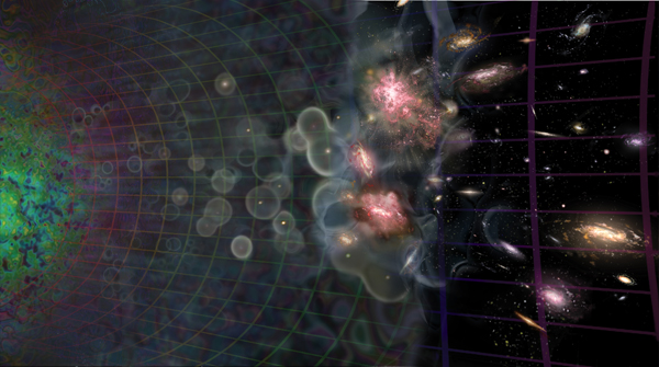
Artist’s illustration of the reionization of the universe (time progresses left to right), in which ionized bubbles that form around the first sources of light eventually overlap to form the fully ionized universe we observe today. [Avi Loeb/Scientific American]
To learn about the early production of light in the universe, our best bet is to study in detail the earliest luminous sources — stars, galaxies, or quasars — that we can hunt down. One ideal target is the galaxy COSMOS Redshift 7, known as CR7 for short.
Targeting CR7
CR7 is one of the oldest, most distant galaxies known, lying at a redshift of z ~ 6.6. Its discovery in 2015 — and subsequent observations of bright, ultraviolet-emitting clumps within it — have led to broad speculation about the source of its emission. Does this galaxy host an active nucleus? Or could it perhaps contain the long-theorized first generation of stars, metal-free Population III stars?
To determine the nature of CR7 and the other early galaxies that contributed to reionization, we need to explore their gas and dust in detail — a daunting task for such distant sources! Conveniently, this is a challenge that is now made possible by ALMA’s incredible capabilities. In a new publication led by Jorryt Matthee (Leiden University, the Netherlands), a team of scientists now reports on what we’ve learned peering into CR7’s interior with ALMA.
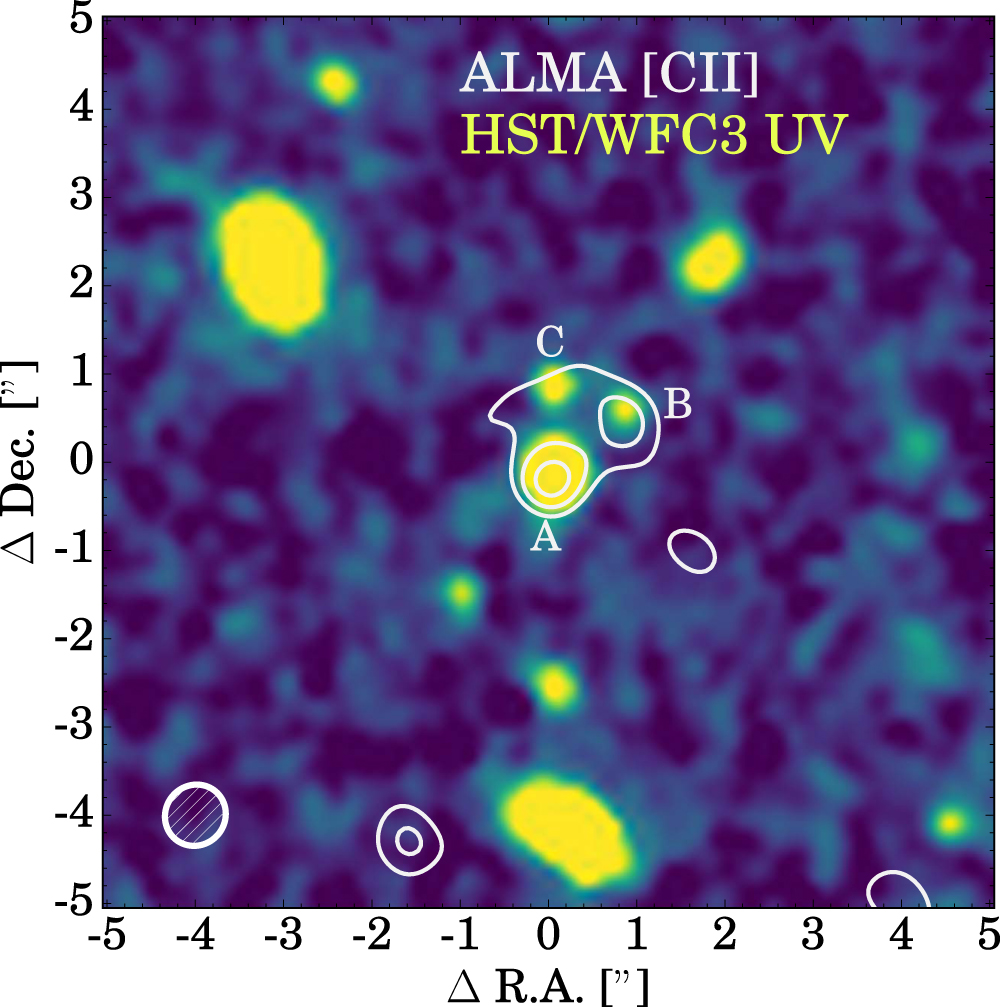
ALMA observations of [C II] (white contours) are overlaid on an ultraviolet image of the galaxy CR7 taken with Hubble (background image). The presence of [C II] throughout the galaxy indicate that CR7 does not primarily consist of metal-free gas, as had been previously proposed. [Matthee et al. 2017]
Metals yet No Dust?
Matthee and collaborators’ deep spectroscopic observations of CR7 targeted the far-infrared dust continuum emission and a gas emission line, [C II]. The authors detected [C II] emission in a large region in and around the galaxy, including near the ultraviolet clumps. This clearly indicates the presence of metals in these star-forming regions, and it rules out the possibility that CR7’s gas is mostly primordial and forming metal-free Pop III stars.
The authors do not detect far infrared continuum emission from dust, which sets an unusually low upper limit on the amount of dust that may be present in this galaxy. This limit allows them to better interpret their measurements of star formation rates in CR7, providing more information about the galaxy’s properties.
Lastly, Matthee and collaborators note that the [C II] emission is detected in multiple different components that have different velocities. The authors propose that these components are accreting satellite galaxies. If this is correct, then CR7 is not only a target to learn about early sources of light in the universe — it’s also a rare opportunity to directly witness the build-up of a central galaxy in the early universe.
Citation
J. Matthee et al 2017 ApJ 851 145. doi:10.3847/1538-4357/aa9931


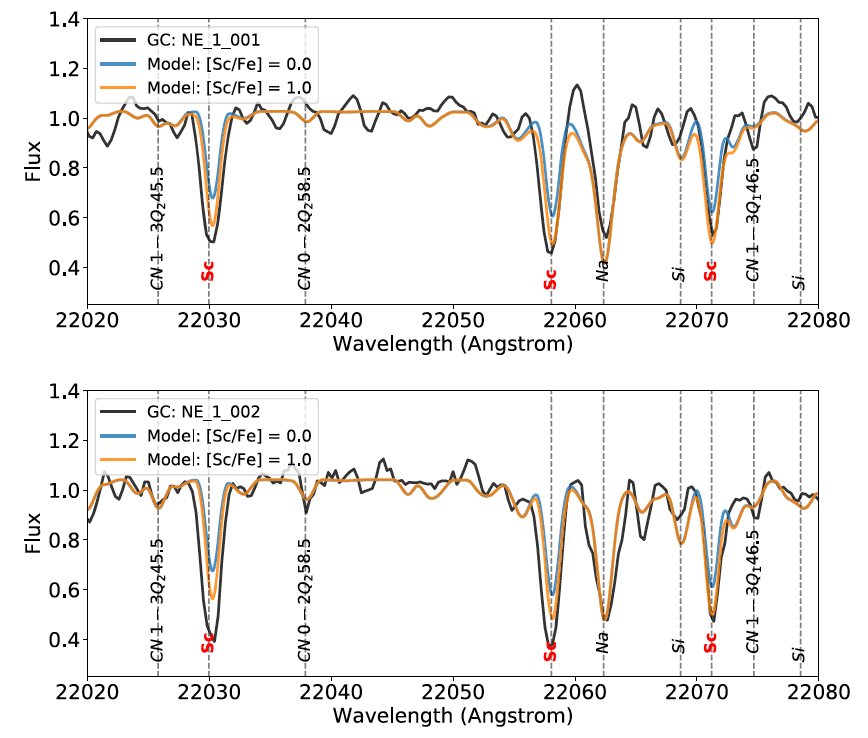
![[Sc/Fe] trend](https://aasnova.org/wp-content/uploads/2018/03/Do18Fig4.png)


