Features Archives - Page 57 of 114

Features RSS

30 September 2020

The Link Between Black Holes and Their Galaxies

The size of a supermassive black hole seems to track with the size of its host galaxy. But is this a statistical fluke, or is there a physical reason for the connection? Recent modeling provides new clues.

Growing Together

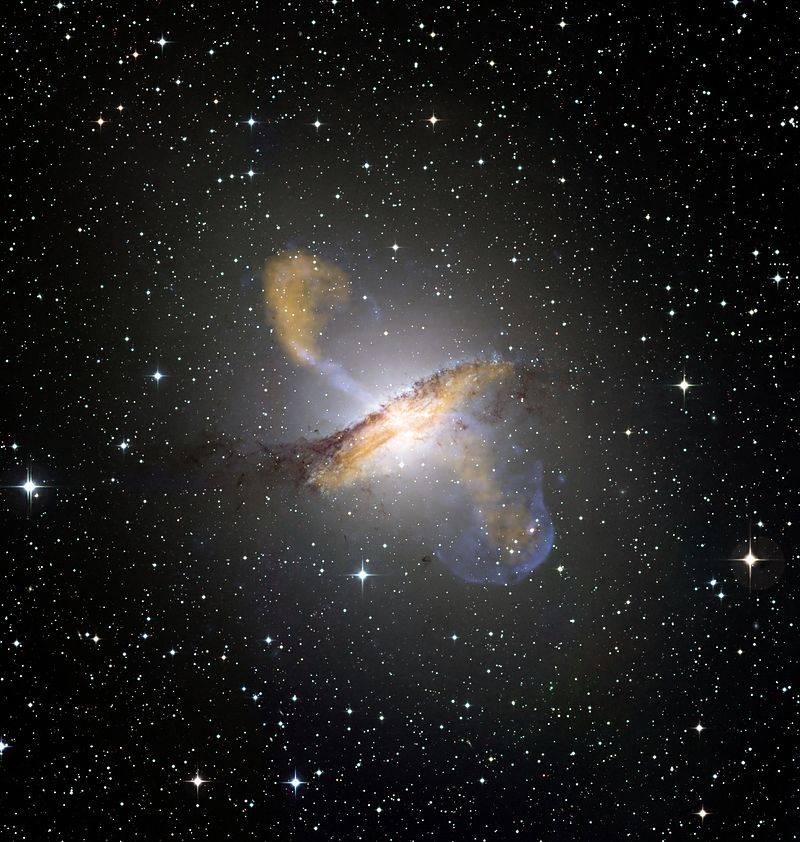
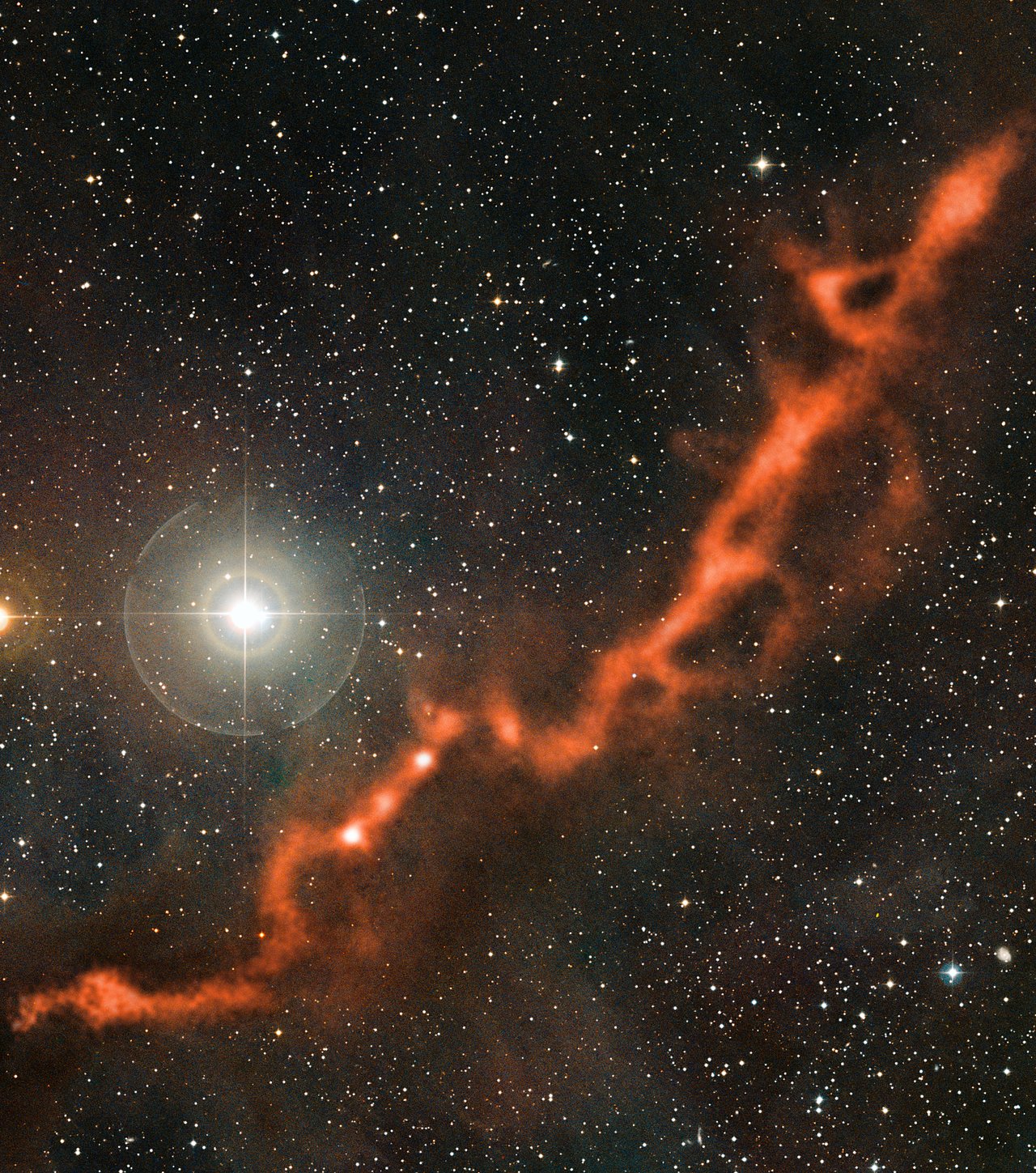
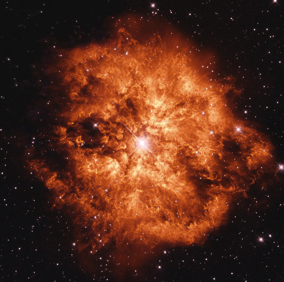
Composite image of Centaurus A, a galaxy whose appearance is dominated by the large-scale jets emitted by the supermassive black hole at its center. [ESO/WFI (Optical); MPIfR/ESO/APEX/A.Weiss et al. (Submillimetre); NASA/CXC/CfA/R.Kraft et al. (X-ray); CC BY 4.0]

The supermassive black holes — black holes of millions to tens of billions of solar masses — that lurk at the active centers of galaxies have a peculiar quirk: their masses correlate with the stellar masses of their hosts. This means that the larger a galaxy is, the larger we can expect its central black hole to be.

But why the connection? How can the black hole know about the galaxy size around it, and vice versa? There are a few proposed explanations for the correlation between central-black-hole mass and its host galaxy’s stellar mass:

It’s caused by active galactic nucleus (AGN) feedback.
In this scenario (recently described here), jets and winds from the accreting black hole can both trigger star formation and quench it by expelling extra gas — star-formation fuel — from the galaxy. This feedback causes the rate of star formation to roughly track the rate of black hole accretion.
It’s caused by black-hole growth and galaxy star formation both relying on the same fuel source.
If black-hole growth and galactic star formation both arise from the same source of fuel, then these two growths should correlate even if they don’t influence each other. One example of a fuel source that could cause sudden growth is a wet merger — the collision of two galaxies rich in gas.
It’s simply a consequence of statistics, and not caused by a physical mechanism.
A theorem known as the central limit theorem suggests that the correlation we observe could arise naturally as a statistical consequence of building up galaxies hierarchically from smaller structures over time. In this scenario, there’s no physical connection between the black hole and its host galaxy — it’s all statistics.

It’s a Matter of the Model

To test which of these explanations is most likely, we need to combine models with observations. A new study led by Xuheng Ding (University of California, Los Angeles) recently set out to do so.

Plots showing the correlation between black hole mass (M_BH) and stellar mass of the host galaxy (M_*. The actual observations are plotted in orange. The blue dots in the top plot show the simulated correlation from the hydrodynamic simulation; the green dots in the bottom plot show the simulated correlation from the semianalytic model. The hydro simulation provides a better match to the data. [Adapted from Ding et al. 2020]

Ding and collaborators first compiled observations of a sample of 32 accreting supermassive black holes and their host galaxies. The sample is from the redshift range 1.2 < z < 1.7, a time in our universe’s history when most supermassive black holes acquired their mass.

The authors then compared these data to the outputs of two state-of-the-art models: a hydrodynamic simulation that focuses on AGN feedback, and a semianalytic model that is especially sensitive to wet galaxy-merger events.

Connecting via Feedback

The results of the authors’ models — in particular, the tightness of the modeled correlation between black-hole and galaxy size across redshifts — strongly support a physical mechanism driving the connection, rather than it being a consequence of statistics.

Of the two models, the hydrodynamic simulation better reproduced the scatter of the correlation, suggesting that AGN feedback may indeed be the driver ensuring that supermassive black holes grow at the same rate as their host galaxies. Observations out to higher redshifts — which may be possible with the upcoming James Webb Space Telescope — will help us further tease out the explanation for this intriguing link.

Citation

“Testing the Fidelity of Simulations of Black Hole–Galaxy Coevolution at z ~ 1.5 with Observations,” Xuheng Ding et al 2020 ApJ 896 159. doi:10.3847/1538-4357/ab91be

23 September 2020

New Molecules from GOTHAM

What as-yet unidentified molecules lurk in the dark clouds of our nearby universe? Answering this requires observation, experiment, and theory — and GOTHAM is on the case.

The Search for New Chemistry

Another view of the Taurus Molecular Cloud, captured here in millimeter wavelengths by the APEX telescope. [ESO]

In the census of the molecular makeup of our universe, the interstellar medium (ISM) is the best target for diversity: we’ve spotted just over 200 different molecules in our galaxy’s ISM. We expect that there are many more out there, however — and identifying where these different molecules are found will help us to understand when and how they form.

To this end, a team of scientists is undertaking the GOTHAM project: a radio search of a cold, dark cloud located 450 light-years away called the Taurus Molecular Cloud 1 (TMC-1). This chilly cloud has not yet collapsed to form a star, providing us with an opportunity to identify new molecules that are able to form in a cold, pre-stellar environment.

Hiding in Slow Motion

But the hunt for molecules in a cold, dark cloud is challenging! We generally identify molecules by searching for their signature transition lines in ISM spectra. But in cold clouds, molecules aren’t moving much, which makes their spectral lines very narrow. This means that we need extremely high-spectral-resolution telescopes to be able to identify them. Fortunately, GOTHAM leverages the 100-meter Green Bank Telescope (GBT), which is up to the task!

The 100-meter Green Bank Telescope in West Virginia. [NRAO/AUI/NSF]

In a new article led by Brett McGuire (MIT, NRAO, and Center for Astrophysics | Harvard & Smithsonian), a team of scientists details the GOTHAM project and its early science results. This is just one of six new articles that describe the first molecular detections by GOTHAM.

An Attack from All Angles

How does a new molecular detection work? As an example, we can look at GOTHAM’s discovery of propargyl cyanide (HCCCH₂CN) in TMC-1.

First, due to the GBT’s high spectral resolution, the team needed to produce new, fine-detail guides for the forest of spectral lines expected from propargyl cyanide. This required new laboratory measurements of the molecule.

Individual line detections of propargyl cyanide in the GOTHAM data. [McGuire et al. 2020]

Next, the team had to search for these lines in the GBT data. Propargyl cyanide has 3,700 transitions that fall within GOTHAM’s observing range, all contributing to the total flux seen for this molecule. Teasing out these signatures requires complex data analysis.

Finally, after achieving a significant detection of the molecule, the team had to do a sanity check. They conducted simulations of TMC-1 using astrochemical codes and included different channels that could form and destroy propargyl cyanide. They then checked that the abundances they measured for this molecule matched expectations from the simulations.

More Discoveries Ahead

This multi-faceted process has already led to a number of new detections in addition to propargyl cyanide. The detections are announced across a set of six articles — including an additional ApJ Letters publication, in which Ci Xue (University of Virginia, Charlottesville) and collaborators detail the first astronomical detection of isocyanodiacetylene (HC₄NC) and the implications for how this molecule and others like it form in the ISM.

What’s more, all of these new results still only make up 30% of the eventual data that will be collected for the GOTHAM project. There’s plenty more to look forward to in the future as we continue to expand our understanding of the chemistry of the universe around us.

Citation

“Early Science from GOTHAM: Project Overview, Methods, and the Detection of Interstellar Propargyl Cyanide (HCCCH₂CN) in TMC-1,” Brett A. McGuire et al 2020 ApJL 900 L10. doi:10.3847/2041-8213/aba632

“Detection of Interstellar HC₄NC and an Investigation of Isocyanopolyyne Chemistry under TMC-1 Conditions,” Ci Xue et al 2020 ApJL 900 L9. doi:10.3847/2041-8213/aba631

21 September 2020

Taking Stock of Backyard Worlds

We’ve tallied up a lot of the stars and substars that lie within our solar neighborhood, but we’re missing a key population: the coolest, dimmest substar dwarfs that lurk nearby. A citizen science study is now filling in this gap with the discovery of 95 new “backyard worlds.”

A Gap in the Census

Three types of progressively cooler brown dwarfs and their characteristics (click to enlarge). Y dwarfs are the coldest of substars. [NASA/JPL-Caltech/Backyard Worlds]

Stellar classification roughly tracks with star temperature, ranging from the wildly hot and bright O-type stars (which burn at more than 30,000 K) all the way down to dim brown-dwarf substars of T and Y types (which can be nearly as cool as Earth, at just 300 K).

To better understand how stars and substars are distributed across this range, we’ve attempted to take a census of the bodies in our local solar neighborhood and observe their characteristics. The challenge in this lies on the brown-dwarf end: we’ve observed very few of the smallest, coldest substars in our solar backyard, because they’re so dim and hard to spot.

How to Spot a Hidden Substar

The key to finding these lurkers is all-sky surveying at long infrared wavelengths. The Wide-field Infrared Survey Explorer (WISE) is an ideal telescope for the task: this spacecraft has surveyed the entire sky in infrared 14 times over the span of a decade, providing us with a wealth of archived data. By searching for cool, dim objects that move quickly between successive images, we can identify the nearby brown dwarfs that we’ve been missing.

The catch? WISE’s imaging archive contains over 30 trillion pixels! Identifying small, dim, moving objects requires human eyes — a lot of them. It’s definitely time for crowd-sourcing.

A Job for 200,000 Eyes

The citizen science project Backyard Worlds: Planet 9 (which we’ve previously talked about) relies on more than a hundred thousand volunteers to examine WISE images and spot cool, nearby star and substar candidates — and after roughly three years of work, the project has now completed around 1.5 million classifications!

This gif illustrates how Backyard Worlds volunteers identify nearby, cold substars: by looking for objects that move (like the “dipole” and “mover” marked here) between successive WISE images. [Backyard Worlds]

In a recent publication, a team of scientists led by Aaron Meisner (NSF’s NOIRLab) describes the follow-up of some of the most likely nearby, cold brown dwarf candidates from Backyard Worlds with the Spitzer space telescope.

Discoveries in the Data

Full-sky distribution of the 96 Backyard Worlds targets followed up with Spitzer. [Meisner et al. 2020]

Meisner and the Backyard Worlds team used Spitzer to confirm 75 objects as newly discovered members of the solar neighborhood. Their discoveries include:

A number of Y-dwarf candidates. These are the coldest of substars, of which there are only a handful known.
Two new worlds that lie within 30 light-years of the Sun.
Two sources moving faster than 2” per year — a potential indicator that they’re relatively old objects with low metallicity.
A T-dwarf substar that appears to be in a binary with a white dwarf.

Artist’s impression of a brown dwarf orbiting a white dwarf. [NOIRLab/NSF/AURA/P. Marenfeld, Acknowledgement: William Pendrill]

There’s still ~1,500 more Backyard Worlds candidates to be followed up, and many of the team’s discoveries will make excellent targets for future observations and characterization. The continued exploration of these coldest substellar neighbors will help us to bridge the gap between low-mass stars and massive planets, expanding our understanding of the worlds that lurk in our solar neighborhood.

Citation

“Spitzer Follow-up of Extremely Cold Brown Dwarfs Discovered by the Backyard Worlds: Planet 9 Citizen Science Project,” Aaron M. Meisner et al 2020 ApJ 899 123. doi:10.3847/1538-4357/aba633

18 September 2020

Different Views of a Fast Radio Burst

Fast radio bursts are perplexing astrophysical phenomena. As their name suggests, they’re essentially short radio signals, but they pack a surprising amount of energy. More unusual is that some fast radio bursts repeat, while others are one-off events.

Repeating fast radio bursts present an opportunity to study bursts in more detail. So what do we see when we observe a burst at multiple frequencies simultaneously?

FRB 121102, the first fast radio burst found to repeat, was also the first to be localized in the sky. [Gemini Observatory/AURA/NSF/NRC]

A Tendency to Repeat Itself

Fast radio bursts (FRBs) typically last only a few milliseconds, but the strength with which they’re detected suggests that FRBs are produced by extremely energetic processes. What these processes are is an open question. Practically all known FRBs originated outside the Milky Way, though that might no longer be the case.

Some FRBs are known to repeat, allowing for their origin to be pinpointed far more accurately than one-off FRBs. The first known repeating FRB, called FRB 121102, lives in a dwarf galaxy over 2 billion light-years away. FRB 121102 has produced hundreds of bursts since its discovery, and studies have determined that it can be detected at multiple radio frequencies.

A new study led by Walid Majid (Jet Propulsion Laboratory/California Institute of Technology) revisited FRB 121102 using DSS-43, a 70-meter radio telescope in NASA’s Deep Space Network. The goal of this study was to probe FRB 121102’s bursts at higher frequencies than previously studied and to examine the bursts’ appearance in broadband observations.

The radio telescope DSS-43, which is located in Canberra, Australia. [NASA]

Only One Right Frequency?

Broadband observations of FRBs provide spectra of the bursts, and spectra are extremely useful. In the case of FRBs, spectral features could either be caused by the mechanism of the burst itself, or they could instead have been added as the signal propagated through the host environment, across intergalactic space, and then through the Milky Way to reach us.

Majid and collaborators observed FRB 121102 with DSS-43 for nearly six hours on September 19, 2019. The observations were centered at 2.25 (S band) and 8.36 gigahertz (X band) with usable bandwidths of ~100 and ~430 megahertz respectively. Six bursts were observed in this time — but they were only seen in the lower-frequency S band!

The brightest burst observed from FRB 121102 as seen in the S band (bottom panel) and not seen in the X band (middle panel). The top panel shows the strength of the burst signal in the S band (black line) and the X band (grey line) as the signal-to-noise ratio versus time. In the middle and bottom panels, the signal is shown as frequency versus time, with dark areas corresponding to the burst. The time unit is milliseconds. [Adapted from Majid et al. 2020]

It All Depends on How You Look at It

The lack of a high-frequency detection for FRB 121102 is interesting, especially since the X band had a larger bandwidth than the S band. Does this frequency dependence provide insight into the FRB emission mechanism? Or does it only arise as the signal propagates to us?

Majid and collaborators explored the possibility that scintillation in our galaxy could be responsible for the lack of visible activity in the X band. In the context of FRBs, galactic scintillation is the observation of multiple bursts at various frequencies, caused by burst photons interacting with material in the Milky Way. The authors show that galactic scintillation can’t account for FRB 121102’s observations, suggesting the frequency dependence may have more to do with intrinsic properties of the emission mechanism or properties of the FRB’s host galaxy.

As with most things in astronomy, more observations are required. Wajid and collaborators concluded that dense, multi-frequency observations of FRB 121102 would go a long way to understanding its behavior. And so the mystery of FRBs continues!

Citation

“A Dual-band Radio Observation of FRB 121102 with the Deep Space Network and the Detection of Multiple Bursts,” Walid A. Majid et al 2020 ApJL 897 L4. doi:10.3847/2041-8213/ab9a4a

16 September 2020

Forecasting Eruptions of Solar Flares

Can we tell when a solar flare will lead to a potentially hazardous eruption of plasma from the Sun? A new look at hundreds of past solar flares may provide some clues.

Belches from the Sun

A large solar flare may or may not be accompanied by a violent ejection of matter in a CME. [NASA/SDO]

Two of the most energetic phenomena in our solar system are solar flares and coronal mass ejections (CMEs). While both are explosions produced in active regions on the Sun, they are distinctly different: solar flares are intense bursts of radiation spanning the electromagnetic spectrum, whereas CMEs are violent, directed eruptions of hot, magnetized plasma — sometimes containing more than a billion tons of matter — into space. While the two phenomena sometimes arise hand in hand, this is not always the case.

The Earth’s magnetic field does a good job of protecting us from the greatest impact of these eruptions, but a CME directed at Earth still has the potential to be hazardous to our technology and communications systems, as well as to any unshielded life (such as astronauts on a lunar mission). Scientists are therefore interested in better understanding which solar flares are likely to be eruptive — i.e., accompanied by a CME — and which ones will instead be confined.

Top: For active regions with low magnetic flux, more flares tend to be eruptive (blue), whereas for active regions with high magnetic flux, more flares tend to be confined (red). Bottom: The proportion of eruptive flares (P_E) decreases with increasing active region magnetic flux. [Adapted from Li et al. 2020]

A Decade of Activity

To this end, a team of scientists led by Ting Li (Chinese Academy of Sciences) recently constructed an extensive catalog of large (M- and X-class) solar flares and associated CMEs observed in 2010–2019 — a time period that spans nearly the entirety of the Sun’s most recent solar activity cycle.

The team then analyzed the 322 resulting flares and cataloged them as either eruptive or confined, depending on whether or not there was an associated CME. Finally, Li and collaborators analyzed the properties of the active regions from which the flares and CMEs arose.

Exercising Magnetic Restraint

Li and collaborators found an anticorrelation between the total magnetic flux of active regions and the proportion of eruptive flares. That means that the active regions with especially small magnetic fluxes were very likely to have flares with accompanying CMEs, whereas the active regions with especially large magnetic fluxes were more likely to have confined flares with no eruptions.

The critical decay index height vs. active region magnetic flux for eruptive (blue) and confined (red) flares shows that regions with more magnetic flux are also more confined. [Adapted from Li et al. 2020]

Why? Perhaps counterintuitively, the stronger magnetic flux actually helps to hold back the flares, preventing them from breaking out and expelling matter in a CME. The authors find additional evidence supporting this picture: the critical decay index height — a measure of how quickly the magnetic field drops off with height — indicates that the active regions with greater flux also have stronger confinement.

Space Weather Predictions

Li and collaborators’ publicly available catalog and results provide us with valuable clues to help forecast CMEs in association with large flares. In addition, these outcomes could have implications beyond our own solar system: they may help us to better understand the flares we’ve witnessed from other stars and even assess the potential habitability of their planets. As we learn more, future solar and stellar belches may become just a little less unpredictable.

Citation

“Magnetic Flux of Active Regions Determining the Eruptive Character of Large Solar Flares,” Ting Li et al 2020 ApJ 900 128. doi:10.3847/1538-4357/aba6ef

Illustration of a space probe with two sets of circular solar panels in the foreground of a small, rocky body.

11 September 2020

A Satellite for Eurybates

Next year, the Lucy space probe will launch on a journey to visit several asteroids in our solar system. One of its destinations, 3548 Eurybates, has recently been discovered to harbor a satellite — providing Lucy with a new target to explore.

A Trojan Population

Animated figure illustrating the orbits of the inner planets, Jupiter (orange disk and orbit), and Jupiter’s trojan asteroids (green disks). The trojans fall into two camps: the Greek camp (the cluster leading Jupiter) and the Trojan camp (the cluster trailing Jupiter). [SwRI]

In astronomy, trojans refers to small bodies that share the orbit of a larger one, residing in stable orbits that either lead or trail the large body. Jupiter provides a prime example of this phenomenon: roughly a million trojan asteroids trace the same path as the giant planet, clumping together into one cluster ahead and one behind Jupiter.

The Jupiter trojans are ancient vestiges of our solar system’s formation — leftover building materials from the construction of the outer planets. Scientists hope that by examining the composition, structure, and dynamics of these time capsules, we’ll learn more about the history of our solar system and the origin of organic materials on Earth.

Getting Up Close and Personal

So far, we’ve detected around 7,000 Jupiter trojans, and we now hope to get a better look at these small, distant bodies. This is where Lucy comes in: this upcoming NASA space probe, slated to launch in October 2021, will fly by six different Jupiter trojan asteroids over the span of six years (2027–2033), providing us with up-close views of these fossils of planet formation.

To prepare for Lucy’s launch, the next step is to characterize the mission’s targets, thereby ensuring that we can plan the spacecraft’s route and observing schedule effectively and efficiently. To this end, a team of scientists led by Keith Noll (NASA Goddard SFC) recently examined one of Lucy’s targets, the trojan asteroid 3548 Eurybates, using the Hubble Space Telescope — and they found more than they bargained for.

This 2” x 2” view of Eurybates from Hubble in January 2020 confirmed the presence of a satellite, identified here by a green circle. [Adapted from Noll et al. 2020]

Pixel Hunting

Noll and collaborators first spotted hints of a satellite body near the 64-kilometer-diameter Eurybates in two sets of Hubble images from September 2018. A 1.7-pixel blip was visible next to Eurybates in both observations, and it shifted location between the two images — an indication this was a blip worth follow-up.

But it’s tough to get follow-up time on one of the world’s most popular telescopes! The team was granted just three opportunities with Hubble to try to confirm this possible satellite. The first two attempts, made in December 2019, failed — the satellite was likely too close to Eurybates to be resolved. But in the third set of observations, the blip reappeared — a faint observation that allowed Noll and collaborators to confirm the presence of a ~1.2-km satellite for Eurybates.

Time to Study Some Collisions

The relative size of known satellite/asteroid pairs in the solar system, plotted against their orbital distance. Symbol sizes are proportional to satellite diameter. Eurybates (blue symbol) is one of the smallest and most distant primaries for which a satellite has been detected from an Earth-based telescope. Click to enlarge. [Noll et al. 2020]

Noll and collaborators use their three detections to place early constraints on the orbit of the satellite and compare it to other known asteroid satellites in our solar system. The relative size of this satellite is remarkably tiny — it’s just 1.9% the size of Eurybates!

The properties of this system suggest the satellite was formed from Eurybates by a collision — providing us with a golden opportunity to study a collisional satellite at close range. With seven years to go before Lucy’s close encounter with Eurybates, we’ve got time to learn more and prepare!

Bonus

Curious how Lucy’s going to manage to visit six different targets, all in one journey? Click below to check out a video from SwRI (or visit the SwRI website directly, if it doesn’t play in your browser) that shows Lucy’s complex planned orbit.

Citation

“Detection of a Satellite of the Trojan Asteroid (3548) Eurybates—A Lucy Mission Target,” K. S. Noll et al 2020 Planet. Sci. J. 1 44. doi:10.3847/PSJ/abac54

9 September 2020

An Update on Fast Radio Bursts: New Discovery in Our Own Galaxy

Have we recently spotted the first equivalent of a fast radio burst (FRB) — a mysterious and brief extragalactic flash of radio emission — in our own galaxy? Some astronomers think so, and argue that the new discovery solidifies the connection between these exotic radio bursts and powerfully magnetized neutron stars.

Origin of a Burst

Artist’s impression of telescopes observing an extragalactic fast radio burst. [CSIRO/Andrew Howells]

Observations of bright, millisecond-duration, extragalactic radio flashes continue to pile up, yet the cause of these odd transients remains uncertain. One popular theory: FRBs may be somehow connected to the birth or evolution of magnetars, neutron stars threaded with especially strong magnetic fields.

There’s plenty of evidence pointing to magnetars as the source of FRBs, from polarization measurements that suggest FRB sources are strongly magnetized, to localizations of several FRBs to star-forming regions typical of magnetar environments. And some magnetars, known as soft gamma-ray repeaters (SGRs), emit repeated high-energy flares and bursts across their lifetime — another sign of volatility that could tie into the FRB picture.

But there’s a major challenge to the magnetar model for FRBs: we’ve never observed radio emission remotely similar to an FRB coming from a magnetar in our own galaxy.

…that is, until now.

A Missing Link Found?

In a new study led by Sandro Mereghetti (INAF, Italy), scientists have reported the detection of a series of bright X-ray bursts from the magnetar SGR 1935+2154 using the International Gamma-Ray Astrophysics Laboratory (INTEGRAL) spacecraft.

The X-ray light curve from INTEGRAL (black line) is shown here with the positions of the associated radio pulses (orange line) marked for comparison. The inset box shows the brightest part of the burst. Click to enlarge. [Mereghetti et al. 2020]

In itself, this announcement might not have been newsworthy — but the observed X-ray bursts from this known magnetar were also accompanied by a very bright millisecond radio burst detected by the Canadian Hydrogen Intensity Mapping Experiment (CHIME) and the Survey for Transient Astronomical Radio Emission 2 (STARE2) radio telescopes.

The radio burst exhibits similar structure to the associated X-ray burst from the magnetar, occurred at roughly the same time, and is within a factor of 10 of the energy of some extragalactic FRBs. These clues strongly suggest that SGR 1935+2154’s outburst may be the missing link that connects magnetars with FRBs.

Pinpointing Production

Can we use these new observations of SGR 1935+2154 to narrow down models of FRB production?

The existence of a second, rare population of magnetars with stronger magnetic fields and higher activity levels could explain a number of properties of the FRBs we’ve observed. As an example, the observed rates of repeating and non-repeating FRBs can be reproduced with the authors’ two-population model. [Adapted from Margalit et al. 2020]

In another recent study, Ben Margalit (NASA Einstein Fellow at UC Berkeley) and collaborators use the new data from this source first to argue that there must be two different populations of magnetars: “ordinary” magnetars like SGR 1935+2154 and other galactic magnetars, and more active but shorter lived magnetars that are responsible for cosmological FRBs. The latter population may form through different channels than galactic magnetars.

Margalit and collaborators also use the radio and X-ray observations from SGR 1935+2154 to evaluate specific magnetar emission mechanisms, providing constraints on models of how these energetic flashes are produced.

SGR 1935+2154 may have more X-ray and radio activity in store for us in the future, so you can bet we’ll be keeping an eye on it. With any luck, upcoming observations will help us to further address the mystery of FRBs — right here in our own galaxy.

Citation

“INTEGRAL Discovery of a Burst with Associated Radio Emission from the Magnetar SGR 1935+2154,” S. Mereghetti et al 2020 ApJL 898 L29. doi:10.3847/2041-8213/aba2cf

“Implications of a Fast Radio Burst from a Galactic Magnetar,” Ben Margalit et al 2020 ApJL 899 L27. doi:10.3847/2041-8213/abac57

4 September 2020

History as Told by a Merger Background

To know the rate of binary black hole mergers over the lifetime of the universe is to know more about the universe’s evolution. For instance, how were binary black holes first created? Did ancient stars in the early universe play a role? And where does chemical composition come into the picture?

But before all that, we first need to answer this question: how do you even determine the history of binary black hole mergers?

Have Data, Do Science!

A view of the Virgo interferometer. [The Virgo Collaboration/CCO 1.0]

Discoveries like the one announced this week illustrate how gravitational-wave observatories like the Laser Interferometer Gravitational-wave Observatory (LIGO) and the Virgo interferometer have pushed the study of binary black hole (BBH) mergers from theory into observation. However, we still haven’t entered an era where BBH mergers are commonplace. This means that it’s hard to do studies that need large ensembles of mergers to make definitive conclusions — like measuring how the rate of BBH mergers changes over the lifetime of the universe.

Another problem is that gravitational-wave observatories can only probe a relatively small volume of the universe. Models have suggested that historical rates of BBH mergers peak at a distance that’s outside the range of current observatories, so what’s to be done?

Two different example models of merger rates versus redshift. Here the peak merger redshift is seen around z ~ 2, and the growth of the low-redshift merger rate is described with a factor called α. [Callister et al 2020]

Redshifts and a Gravitational-wave Background

A lot, it turns out! In a new study, a group of researchers led by Tom Callister (Flatiron Institute) used LIGO/Virgo gravitational-wave data to put observational constraints on the evolving rate of BBH mergers. A special feature of their study was that they didn’t just consider directly observed mergers — they also looked at the overall background of gravitational-wave signals that observatories can detect.

To be specific, Callister and collaborators were attempting to measure how the rate of BBH mergers changes with redshift. LIGO/Virgo can detect individual mergers out to a redshift of z ≲ 1, but models suggest that BBH merger rates peak somewhere between z ~ 2 (about 10 billion years ago) and z ~ 4 (nearly 12 billion years ago). So, Callister and collaborators decided to combine information from individual BBH mergers (“shouts”) with the limits we have on the gravitational-wave background created by more distant, undistinguished mergers (“murmurs”).

In the Background No More

Predicted merger rate (in mergers per cubic gigaparsec per year) versus redshift based on ~1 year of simulated Advanced LIGO observations at design sensitivity. The solid line is the “true” merger rate used to generate the simulations; the other lines show the results from different mock detections. The top plot is based solely on directly observed mergers, while the bottom plot includes the gravitational-wave background in the analysis. Click to enlarge. [Callister et al 2020]

The primary quantities of interest in this study were the redshift at which mergers peak (z_p) and how quickly the merger rate grows as we look farther away in the local universe (quantified by the exponent α in the plot shown above).

By combining direct merger detections with upper limits on the gravitational-wave background for the first time, Callister and collaborators were able to rule out certain combinations of peak merger redshifts and local merger growth rates. In particular, they reject combinations of z_p ≳ 1.5 and α ≳ 7, limiting the merger rate to peak more recently than ~9 billion years ago if the local growth rate of BBH mergers is large.

So what’s next? With the upgraded Advanced LIGO and other gravitational-wave observatories coming online soon, many more mergers will be within reach. The limits the authors have already established are just a start; the authors also show that the upgraded Advanced LIGO may make it possible to pin down the peak merger redshift with certainty. So keep your eyes peeled!

Citation:

“Shouts and Murmurs: Combining Individual Gravitational-Wave Sources with the Stochastic Background to Measure the History of Binary Black Hole Mergers,” Tom Callister et al 2020 ApJL 896 L32. doi:10.3847/2041-8213/ab9743

2 September 2020

LIGO/Virgo’s Newest Merger Defies Mass Expectations

Been waiting for new signals to be parsed from LIGO/Virgo’s third observing run data? Wait no longer! The latest detection announced in Physical Review Letters and ApJ Letters is big news — both figuratively and literally. The two black holes that merged in GW190521 are the most massive we’ve observed yet, and this has major astrophysical implications.

The Signal

Most recent version of the “stellar graveyard”, a plot that shows the masses of the different components of observed compact binary mergers. GW190521, seen at the top center, is more massive than any other binary merger we’ve observed. Click to enlarge. [LIGO-Virgo/Northwestern U./Frank Elavsky & Aaron Geller]

On May 21, 2019, the LIGO/Virgo gravitational-wave observatories detected a strong signal in all three of their detectors. After the conclusion of the observing run and careful analysis of the waves, the collaboration is now announcing GW190521 as an official detection of the inspiral and merger of two extremely massive black holes.

This signal is unique, record-breaking, and extremely intriguing for two reasons. First, the final product of the merger is ~142 times the mass of the Sun, which places it firmly in the category of elusive intermediate-mass black holes. And second, the two merging black holes had masses of ~85 and ~66 solar masses, which virtually guarantees that at least one of them falls into the so-called pair-instability mass gap.

A Decidedly Intermediate Size

Let’s unpack these things, starting with the final product.

The black holes astronomers have thus far observed in the universe fall into two primary categories: stellar-mass black holes (on the order of ~10 solar masses), and supermassive black holes (millions to tens of billions of solar masses).

Intermediate-mass black holes (IMBHs) should exist as a bridge between the two, spanning the range of 100–100,000 solar masses. Until now, however, evidence for these bodies has been slim: only a few candidates, all with masses at the upper end of the IMBH mass range, have been identified.

The detection of GW190521’s 142-solar-mass final product therefore marks a major discovery in a black-hole-mass desert. It confirms not only that IMBHs do exist, but also that they can be formed by the merger of two smaller black holes.

Illustration of the steps of a hierarchical merger, in which four stellar-mass black holes combine in pairs to eventually form a single, large black hole. [LIGO/Caltech/MIT/R. Hurt (IPAC)]

Polluting the Mass Gap

Stellar-mass black holes form when a massive star evolves and collapses at the end of its lifetime. But there’s an instability that’s thought to get in the way for some stars, expelling mass and preventing black holes of a certain range of masses from forming.

This forbidden pair-instability mass gap lies roughly between 65 and 120 solar masses — and yet the masses of the merging black holes in GW190521 fall squarely within that range!

How can this be? The LIGO/Virgo collaboration outlines a few possible ways to defy the mass gap:

Second-generation black holes
Black holes that formed from the merger of two smaller black holes (instead of from the collapse of a star) can lie within the mass gap. GW190521 might be the result of four stellar-mass black holes undergoing progressive hierarchical mergers to eventually form an intermediate-mass black hole.
Stellar mergers in young star clusters
In some scenarios, the merger of an evolved star with a main-sequence companion can create a giant star with an oversized envelope. This type of star could collapse directly into a black hole that lies in the mass gap.
Artist’s illustration of two merging black holes embedded in the gas disk surrounding a supermassive black hole. [Caltech/R. Hurt (IPAC)]
Black-hole mergers in the disks of active galactic nuclei
The disk of material that feeds the supermassive black hole at the center of an active galaxy may host tens of thousands of stellar-mass black holes. Trapped in the disk, these smaller black holes can more efficiently accrete material and merge, providing an avenue for rapid growth into mass-gap sizes.

Going Forward

We can’t yet be sure whether GW190521 represents a new kind of black hole binary, or if it’s simply the upper-mass end of the population we’ve already observed. But this will soon change, as upgrades to the LIGO/Virgo network’s sensitivity should allow for the detection of several hundreds of mergers per year, reaching ever higher redshifts. And next-generation ground- and space-based detectors will soon provide an additional perspective.

With the surprising discoveries of GW190521, one thing is clear: the paradigm shifts from gravitational-wave astronomy are only just beginning.

Citation

“Properties and Astrophysical Implications of the 150M_☉ Binary Black Hole Merger GW190521,” Abbott et al 2020 ApJL 900 L13. doi:10.3847/2041-8213/aba493

28 August 2020

A Stellar Pinwheel at a New Wavelength

Spiral galaxies are one thing — but some spiral patterns in the sky are created much closer to home, arising from stars instead! A recent study explores a stellar pinwheel spotted around an unexpected source.

Monster Stars

The powerful winds of a lone Wolf-Rayet star — like WR 124, seen in this actual Hubble image — can inflate a stunning nebula as the star loses mass. [ESA/Hubble & NASA / Judy Schmidt]

Even on the already dramatic scale of massive, evolved stars, Wolf-Rayet stars are extreme.

These monsters are in the final stages of their evolution, doomed to end their lives soon as violent supernovae. Until then, Wolf-Rayet stars are here for us to observe: scalding hot — with surface temperatures that range from 30,000 K to 210,000 K — and enthusiastically shedding mass via powerful stellar winds that can reach speeds of up to 3,000 km/s (that’s 6.7 million miles per hour).

Putting on a Show

Wolf-Rayet stars can create quite the spectacle, generating stunning nebulae even when isolated. But put them in a binary pair with another hot, massive star? Then you get something else entirely. In particular, scientists have found multiple examples of Wolf-Rayet binaries producing astonishing spiral pinwheel patterns of dust, visible in the infrared.

Schematic showing the formation of a spiral around a binary consisting of a massive star and a Wolf-Rayet star, both emitting powerful stellar winds. Click to enlarge. [Gemini Observatory/Jon Lomberg]

How does this work? Where the strong winds of the Wolf-Rayet star and its massive companion collide, a plume of dense gas and dust is produced that gets carried outward with the Wolf-Rayet wind. As the pair of stars orbits, the dust plume forms an ever-expanding spiral extending from the binary.

Pinwheels Tied to Type?

Wolf-Rayet stars are identifiable by characteristic broad emission lines. From their spectra, these stars can be classified into two main subcategories: those with strong carbon and helium lines (WC subtype) and those with strong nitrogen and helium lines (WN subtype).

Infrared pinwheel structures have only ever been spotted around binaries that contain WC-subtype stars — likely because WC winds facilitate infrared-emitting dust formation in the shocked region where the Wolf-Rayet winds collide with those of its binary companion, whereas WN winds do not.

The top panel shows a false-color radio image of WR 147, captured with the Jansky Very Large Array. Can’t make out the spiral? Check out the bottom panel, which is the same image as a contour map, with the pinwheel marked by crosses. The binary lies at the heart of the spiral; the source of emission above the binary is due to an additional, distant stellar companion forming a triple system. [Adapted from Rodríguez et al. 2020]

But now, a team of scientists led by Luis Rodríguez (UNAM Radio Astronomy and Astrophysics Institute; Autonomous University of Chiapas, Mexico) has found an example of a WN-subtype star that’s also created a pinwheel: WR 147. The catch? The pinwheel isn’t visible in infrared; in fact, we can only see it at radio wavelengths.

A Different Emission Mechanism

What’s going on with WR 147? This star is still emitting strong stellar winds that collide with the winds of its companion — but because of its WN subtype, it doesn’t form a dust plume at the collision point. Nonetheless, particles are still being accelerated in the collision zone, and they emit synchrotron radiation, a type of radio emission caused by particles spiraling around magnetic field lines.

Thus, WN-subtype Wolf-Rayet stars can still form pinwheels — we just have to look at radio observations of the systems rather than infrared in order to spot them. This discovery opens the door to significant further exploration of these systems, providing us with the opportunity to probe orbital periods, wind speeds, wind-momentum ratios, and more. You can bet we’ll be looking for more of these spirals in the sky in the future!

Citation

“A Radio Pinwheel Emanating from WR 147,” Luis F. Rodríguez et al 2020 ApJL 900 L3. doi:10.3847/2041-8213/abad9d

Previous 1 … 55 56 57 58 59 … 114 Next