
Spotting a Faint Escaping Atmosphere
Low-density planets struggle to hold on to their atmospheres when they’re blasted with high-energy radiation from a close-by host star. New observations have caught a view of one such escaping atmosphere using a powerful tracer: helium.
Atmosphere on the Run
When a planet orbits close to its star, incoming ultraviolet radiation can heat and puff up the planet’s atmosphere, extending it so far that the gravitational pull of the planet can no longer hold it in. The mass loss that results from this process dramatically shapes the population of short-period exoplanets — so understanding atmospheric escape is critical to our understanding of planetary evolution.
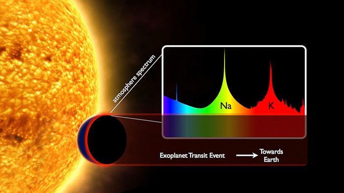
As a star’s light filters through a planet’s atmosphere on its way to Earth, the atmosphere absorbs certain wavelengths depending on its composition. [European Southern Observatory]
In 2018, however, a new discovery provided some hope: the first detection of helium in an exoplanet atmosphere.
Letting Helium Lead
Why is helium helpful? When a low-density planet is pelted with extreme ultraviolet radiation, this can produce a population of helium atoms in the planet’s upper atmosphere that exist in a long-lived excited state. This metastable helium absorbs photons even at the low pressures that accompany high altitudes, creating a prominent absorption feature at the near-infrared wavelength of 1,083 nm.
By hunting for this absorption line — which, since it falls in the infrared, can be observed even through the Earth’s atmosphere using ground-based telescopes — we can probe the extended atmosphere of close-in transiting planets, measuring how much mass the planets are losing through atmospheric escape.
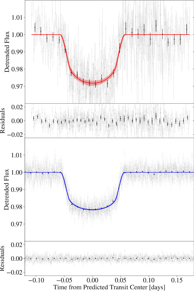
Folded data and best-fit models showing the transit light curve and residuals for HAT-P-18b at 1,083 nm (top) and the corresponding broad-band light curve from TESS (bottom). The transit depth in the helium bandpass exceeds that in the TESS bandpass by roughly half a percent. [Adapted from Paragas et al. 2021]
Loss from a Giant
HAT-P-18 is a K-type star located about 540 light-years away. The star hosts a gas-giant planet, HAT-P-18b, on a close-in, transiting orbit of just 5.5 days. Though the planet is roughly the size of Jupiter, it contains only 20% of Jupiter’s mass — making it very low-density and an excellent target to search for an escaping atmosphere.
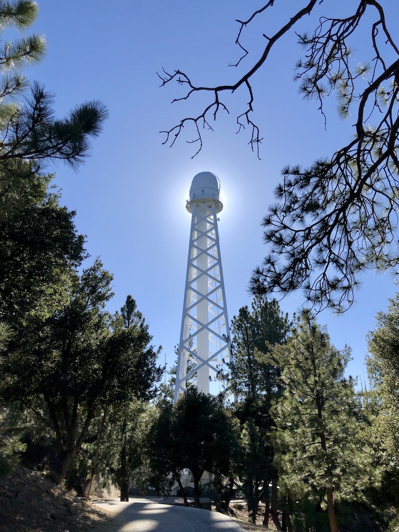
Paragas and collaborators observed two transits of HAT-P-18b with the 200” Hale Telescope at Palomar Observatory in California, using an ultra-narrow band filter centered on the 1,083-nm line. In these observations, the team successfully detected excess helium absorption that allowed them to measure the planet’s escaping upper atmosphere.
By applying wind models to these observations, the authors show that HAT-P-18b is losing less than 2% of its mass per billion years.
HAT-P-18b is one of only a handful of planets whose extended atmosphere has been measured using helium, and it’s the faintest yet. This study therefore demonstrates the effectiveness of using mid-sized, ground-based telescopes to survey planets that lie close in around faint stars, providing a valuable opportunity to learn more about the evolution of this population.
Citation
“Metastable Helium Reveals an Extended Atmosphere for the Gas Giant HAT-P-18b,” Kimberly Paragas et al 2021 ApJL 909 L10. doi:10.3847/2041-8213/abe706


