Features RSS

Black hole with a ring around it that has a tail, which shows the black hole pulling material off a star that's out of the frame.

Tucked away in the deep corners of the universe may lie intermediate-mass black holes: the missing link between supermassive black holes, which sit at the centers of most galaxies, and stellar-mass black holes, which result from supernovae. Could white dwarfs help us find these elusive enigmas? 

Tidal Tale Signs of an Intermediate Black Hole

Though intermediate-mass black holes have been challenging to find, they may reveal themselves when they rip apart a white dwarf and cause a burst of nucleosynthesis, the process that transforms light elements into heavier elements. Modeling the interaction of intermediate-mass black holes with white dwarfs can give us clues to what the electromagnetic signature of these events looks like, which we can then search for with telescopes.  

However, the 3D simulations we’d ideally use for this work are computationally expensive. Modeling these interactions requires looking at timescales from microseconds to hours to capture detailed nuclear physics and massive accretion flows. We also need to model length scales from tens of meters to thousands of kilometers to study hotspots of nuclear ignition as well as track the white dwarf throughout its orbit. Though 3D simulations might capture the physics most accurately, working in 2D reduces the computational cost and eliminates factors that may not be vital to understanding the system as a whole. A team led by Peter Anninos (Lawrence Livermore National Laboratory) simulated these tidally disrupted white dwarfs in 2D to test how well these simulations stack up against their 3D counterparts. 

Three panels on top of each other; top panel shows a line going from the top of the y-axis (value at 0.5) sloped down, hitting the x-axis at 0.5, with a fairly uniform gas density at roughly 4e+04; middle panel shows a line again starting at 0.5 on the y-axis but sloping down more gradually and landing at roughly 6.5 on the x-axis (with just small bumps from 6.0 to 6.5) and a fairly uniform density but a higher density from 6.0 to 6.5 (around 1e+06); bottom panel shows the same as the middle but with a big bump with contours from 6.0 to roughly 7.5 on the x-axis

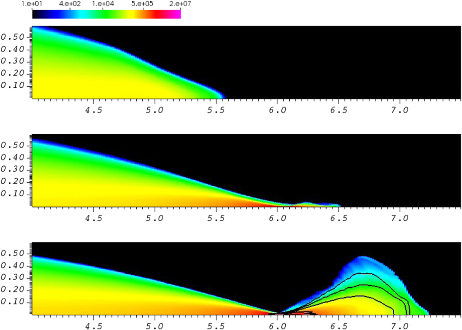
The gas density over time for the 0.15 solar mass helium white dwarf with a fairly strong tidal force. The top panel is at a time of 1.25 seconds, the middle at 1.36 seconds, and the bottom at 1.45 seconds. The color bar represents the density of the gas in g/cm-3. The x and y axes plot distances, which are given in terms of 104 km. [Anninos et al. 2022]

Only Time Will Tell

The team simulated the interaction of a 0.15-solar-mass helium white dwarf and a 0.6-solar-mass carbon–oxygen white dwarf with intermediate-mass black holes at various distances — which correspond to various tidal strengths — and observed the conditions that triggered nucleosynthesis in both helium and carbon–oxygen white dwarf encounters.

After setting the initial conditions at a wide range of spatial scales, the authors ran time forward to see when specific elements were formed and when detonation (the start of nucleosynthesis) occurred. In the various scenarios, helium burned to carbon before detonation occurred, and the rising gas temperature triggered a detonation wave that burned carbon, oxygen, and their byproducts into nickel and iron.

Compression Conclusion

Anninos and collaborators found slight differences between the processes that trigger nucleosynthesis in the different strength interactions. Overall, they concluded that detonation of nucleosynthesis is mainly triggered by adiabatic compression — compression without a change in heat. Their tests between helium and carbon–oxygen white dwarfs showed very little difference in their behavior. 

Top panel: a density from 10^-4 g/cm^3 to 10^8 g/cm^3 with an x-axis from 0 to 2.5 (in units of 1e2) km, and showing a black line that has some spikes around y=10^-2 and around x=0.7, slopes up quickly; Bottom panel: same axes but with all of the colors of lines coming together around x=0.5 to x=1.3

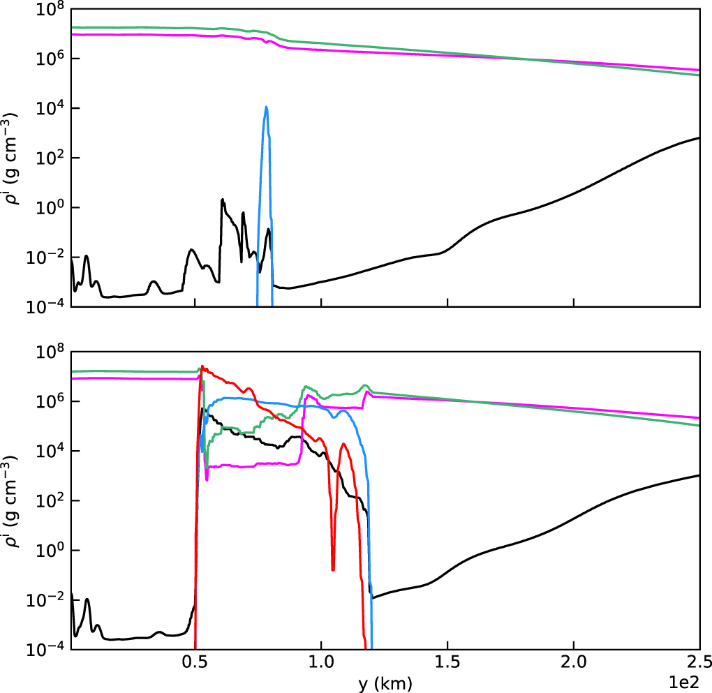
Line profiles of the density of the helium (black), carbon (magenta), oxygen (green), calcium (blue), and nickel (red). The top panel shows densities just before the detonation and the bottom shows after. [Anninos et al. 2022]

The authors’ work reveals that 2D simulations are comparable to those in 3D, specifically for the modeled density and temperature profiles. Understanding the onset of nucleosynthesis in the tidal disruption events of white dwarfs allows us to predict the signature of an intermediate-mass black hole, which may finally lead to the detection of these mysterious objects.  

Citation 

“Resolution Study of Thermonuclear Initiation in White Dwarf Tidal Disruption Events,” Peter Anninos et al 2022 ApJ 934 157. doi:10.3847/1538-4357/ac7b87  

computer visualization of a binary supermassive black hole system

Astronomers study gravitationally linked pairs of black holes to understand how stellar-mass black holes form. What can we learn from black holes that are off kilter from the binaries they belong to?

You Spin Your Way, and I’ll Spin Mine

a diagram illustrating positive and negative effective spin

Top: The black hole spins are aligned with the system’s orbital angular momentum (positive effective spin). Bottom: The black hole spins are misaligned with the system’s orbital angular momentum (negative effective spin). [AAS Nova/Kerry Hensley]

Collecting the gravitational waves from merging stellar-mass black holes allows us get at one of the fundamental questions in high-energy astrophysics: how did the black holes that exist in the universe today come to be? A black hole’s mass and spin hint at whether it formed directly from the collapse of a massive star or through a process called hierarchical merging — the formation of large black holes through successive mergers of smaller ones.

One property we can use to probe the origins of black holes in merging binary systems is the effective inspiral spin parameter, denoted χeff, which is a measure of how aligned the spins of the black holes are with the orbit of the binary pair. In some systems, the black holes spin in the same direction as they orbit, giving the system positive χeff. In others, one or both black holes are tilted, and they spin in directions that are at odds with their orbital motion, giving the system negative χeff. A recent publication searches for the most misaligned black hole binaries to understand the origins of the black holes in the universe today.

plots of the effective spin distribution for binary systems containing one or two black holes formed through hierarchical merging

Theoretical probability distribution functions (top) and cumulative distribution functions (bottom) for the effective inspiral spin parameters (χeff) of binary systems containing one (orange) or two (blue) black holes formed through hierarchical merging. The different lines in the top panel show the effect of different initial black hole spins. [Fishbach et al. 2022]

Monitoring Misalignment

Maya Fishbach (Northwestern University) and collaborators began their investigation by predicting the spins of black holes in binaries in which at least one member formed through hierarchical merging. The team’s calculations showed that hierarchical merging results in a substantial number of black holes with spins misaligned from their direction of orbital motion. Specifically, the team predicted that 16% of black hole binaries would have χeff less than −0.3, regardless of whether one or both members of the binary system arose through hierarchical merging.

With this prediction in hand, Fishbach and coauthors turned to the data, assessing the χeff values of 69 merging black hole pairs in the third Gravitational-wave Transient Catalog (GWTC-3), which is the most recent catalog of gravitational wave events detected by LIGO and Virgo. Depending on the model used to analyze the data, the team found that the maximum proportion of binary systems with χeff less than −0.3 is 4.2%.

Evidence for Meager Mergers

plot of expected number of misaligned binary mergers as a function of total number of events observed and

The expected number of gravitational wave events for systems with χeff less than −0.3 that we expect to observe as a function of the hierarchical merger (HM) fraction and the total number of events observed. [Fishbach et al. 2022]

Given the small fraction of strongly misaligned black hole systems, the team found that hierarchical mergers likely populate no more than 26% of black hole binaries. Intriguingly, only 69% of massive black holes (60 solar masses) are expected to be products of hierarchical merging, meaning that some of these high-mass black holes most likely result from enormous collapsing stars — a finding that has implications for our understanding of stellar interiors and nuclear physics.

Fishbach and collaborators note that if black hole binaries with χeff less than −0.3 aren’t detected in the future, that would point to hierarchical merging being even less common. If the LIGO, Virgo, and KAGRA gravitational wave detectors find no such systems during their next observing runs, the team limits the percentage of black holes formed through hierarchical merging to no more than 2.5%.

Citation

“Limits on Hierarchical Black Hole Mergers from the Most Negative χeff Systems,” Maya Fishbach et al 2022 ApJL 935 L26. doi:10.3847/2041-8213/ac86c4

The logo of the Astropy Project, which is a stylized snake curled into the shape of a spiral galaxy

If producing new results in astronomy research is like constructing a house, different pieces of software used in the process are like the builder’s tools. One of the most fundamental of these tools, a screwdriver of the astronomy world, just got a major update.

The Python Era

Over the past 30 years, the common workflows used to analyze and present scientific findings in astronomy have evolved. While Fortran was the most common programming language discussed in peer-reviewed astronomy publications in the 1990s, IDL overtook this long-leading language to become the dominant method in the early 2000s. Most recently, this top position was usurped again just prior to 2016 when Python became the most-mentioned language. Since its reign began, Python’s popularity has only grown, and now it is regularly used in over 1,000 publications per year.

A plot showing the number of times a given programming language mentioned in refereed astronomy articles per year between 1990 and present. Five languages are shown, and Python has been the most popular since 2016.

A plot illustrating the trends in usage of various programming languages in refereed astronomical literature over time. [The Astropy Collaboration et al. 2022]

One driver for this ascendence in popularity is the ease of creating, modifying, and tweaking major software libraries. In 2013, a loose network of collaborators unveiled one of these libraries that aimed to handle many routine tasks in astronomical research, like unit manipulation, coordinate transforms, and more. Called Astropy, it was quickly adopted by the community, and as of this writing its release publication is the fifth most cited refereed astronomy article from the last decade

In the intervening years, the Astropy Collaboration and the software it maintains have both grown in scope. Astropy now underpins an “ecosystem” of other more specialized astronomy packages, and many new features have been added to the original core. In August of this year, a team of over 100 Collaboration members published the third article in the Astropy series which details their latest efforts and announces the newest major release of Astropy, version 5.0.

New Features

According to the authors, the core Astropy package is designed to stay as broadly applicable to as many subfields of astronomy as possible. As such, most domain-specific updates live in one of more than 50 “affiliated” packages, some of which are maintained by the central Astropy Collaboration, others by independent groups. 

However, there were still several updates deemed useful for the entire community that made it into v5.0, including a new subpackage to handle uncertainties and invoke various statistical distributions, and a new subpackage for manipulating time series data directly within the Astropy environment. Other major additions are listed in Section 2 of the Collaboration’s article.

Collaboration Updates

Besides documenting the new feature additions, the authors also included an update on the governance and health of the Collaboration. Astropy is not maintained by one central institution, but rather by interested members of the community who interact via its GitHub repositories. Until recently, the over 1,500 contributors have worked together without a formal charter, but in fall 2021 the collaboration adopted a more explicit governance structure.

A two-panel plot showing the number of commits to the Astropy core package per month over time on top, and the number of unique Collaboration members submitting those commits on the bottom. Both curves are relatively flat between 2011 and present.

A plot illustrating the number of active collaborators and the number of their additions to the Astropy code base. [The Astropy Collaboration et al. 2022]

Additionally, the Collaboration pursued and acquired several large grants for the first time in its history, both from private foundations and from NASA, which it intends to use to seed longer-term stability.

This useful experiment in open-source, collaborative research code continues to evolve, and further additions are rolled out regularly.

Citation

“The Astropy Project: Sustaining and Growing a Community-oriented Open-source Project and the Latest Major Release (v5.0) of the Core Package,” The Astropy Collaboration et al 2022 ApJ 935 167 doi:10.3847/1538-4357/ac7c74

Full moon against a black sky

Though it is our closest neighbor, the Moon remains partially shrouded in mystery. Under the surface of the Moon lie cryptomaria, remnants of ancient lava flows that were buried during periods of unknown lunar activity. Can radar observations help us map these hidden maria and uncover the secrets of the Moon’s volcanic past?

Title "Moon features you can see from Earth for Northern Hemisphere observers" and different maria and craters labeled

A map of different features on the Moon. [NASA/GSFC/Arizona State University/The Planetary Society]

It’s a Crater…It’s a Highland…It’s…Hidden Lava Flows?

The Moon is full of interesting geological features, from mountains that form the rims of craters to maria left over from ancient lava flows. However, not all of these features lie on the surface: cryptomaria are maria that formed early in the Moon’s history and have been buried by crater ejecta, hiding them from view. Cryptomaria can be mapped using a number of techniques: photographs reveal their locations on the surface (as they’re usually surrounded by dark-halo craters) and spectroscopic analysis shows their characteristic basaltic composition. A team led by Ali Bramson (Purdue University) has taken a new approach to searching for these buried seas: using radar to map their boundaries.  

Top image: 60 degrees S to 60 degrees N latitude by 135 degrees W to 135 degrees E longitude map of the Moon with a small red square circle from ~70 degrees W to 38 degrees W latitude and 60 degrees to 30 degrees S. Bottom: that zoom-in with five areas in boxes with dotted lines labeled #1-#5. Regions of white (cryptomare, Whitten & Head 2015a), light gray (light plaines, Meyer et al. 2020), and yellow (mare, Nelson et al. 2014) are shown.

A map of the estimated areas of cryptomaria from previous studies. [Bramson et al. 2022]

Looking for Cryptomaria in All the Right Places

Researchers use radar to probe below the surface of the Moon by sending radio waves toward the lunar surface and measuring the waves that bounce back. Observing using this approach can help uncover cryptomaria that are buried too deep to have been noticed in visible images and spectroscopic analyses, and it can also reveal ones that have not been exposed by impact craters.  

The team chose the Schiller–Schickard region in order to build on previous volcanic studies, which have used spectroscopy, visible images, and gravity signatures to study the multiple dark-halo craters in the area. Bramson and collaborators study used ground-based radar from the Arecibo and Green Bank telescopes, as well as space-based data from the Lunar Reconnaissance Orbiter Miniature Radio Frequency Instrument (LRO Mini-RF) to observe the region in a new way. 

Putting the “Rad” in “Radar” 

The team used radar at two different frequencies—P-band (430 MHz) and S-band (2380 MHz)—to study the area. Since the two frequencies probe different depths below the surface and structures of different sizes, any differences in the reflected radar signals would indicate similarities or differences between subsurface structure. Bramson and her team looked at the reflected radar signal in five locations and found new cryptomaria outside of previously mapped areas, indicating that the Schiller–Schickard region contains a large network of ancient lava flows. They also used the radar observations to estimate how deep the cryptomaria are buried and found that, in this region, the ancient lava flows are anywhere from ~10 to ~130 meters below the surface. This also shows that the cryptomaria in the region are more extensive than previously thought. If this is true, it could mean that we’re underestimating the amount of cryptomaria beneath the surface of the Moon by more than a factor of two. 

Title: "Interpretation of Schiller Schickard Volcanism. A region (60 degrees to 30 degrees South latitude and 70 degrees to 40 degrees West latitude) showing different colors for Mare (boundaries set by Nelson et al. 2014), very shallow cryptomare, shallow cryptomare, deep cryptomare, and deepest cryptomare (boundaries by Whitten and Head 2015a). Splotches of all colors are shown (along with just gray areas of the Moon)

A map of the depth of cryptomaria detected in the Schiller–Schickard region. [Bramson et al. 2022]

This study only focused on one region where cryptomaria are known to be prevalent, but it shows how useful radar can be in searching for these geologic features. The authors hope that future work will look at other areas where cryptomaria have been hypothesized in order to see if those areas have been underestimated as well.

Citation 

“Burial Depths of Extensive Shallow Cryptomaria in the Lunar Schiller–Schickard Region,” A. M. Bramson et al 2022 Planet. Sci. J. 3 216. doi: 10.3847/PSJ/ac8670

Artist's impression of a binary system containing a massive main-sequence star and a black hole

composite optical, x-ray, and radio image of X-ray binary Circinus X-1

Circinus X-1, shown here in X-ray (blue) and radio (purple) emission overlaid on an optical image, is a binary system containing a main-sequence star and a neutron star, which was discovered because of its bright X-ray emission. [X-ray: NASA/CXC/Univ. of Wisconsin-Madison/S. Heinz et al; Optical: DSS; Radio: CSIRO/ATNF/ATCA]

We’ve detected only a small fraction of the black holes, neutron stars, and white dwarfs that inhabit binary systems. A new research article explores a way to reveal the most elusive of these compact objects.

Searching for Compact Objects

When stars expire, the remnants left behind — black holes, neutron stars, and white dwarfs — are difficult to detect. Black holes emit no light, and tiny neutron stars and white dwarfs shine only weakly compared to stars in their prime. These hard-to-detect compact objects sometimes reveal themselves by accreting gas from a binary companion; as gas spirals toward the object, it forms a superheated disk that blazes in X-rays.

But how do we find compact objects that don’t announce themselves through accretion? In a new publication, Nicholas Sorabella (Lowell Center for Space Science and Technology and University of Massachusetts Lowell) and collaborators show how models can help us identify quiet compact objects in binary systems.

Questing for Companions

Instead of trying to detect faint or invisible binary companions directly, Sorabella and collaborators explored how the presence of an unseen object affects the other component of the binary system: the star. The brightness of a star locked in a binary system with a compact object will change over the course of an orbit for three reasons:

example light curves generated by the model for a binary system containing a sun-like star and a black hole

Modeled light curves for a binary system containing a solar-mass star and a 10-solar-mass black hole with an orbital period of 3 days. The curves show the effects of Doppler boosting (DB), ellipsoidal variations (EV), and self-lensing (SL), as well as their combined effects. Top: orbital eccentricity of 0 (circular orbits); bottom: orbital eccentricity of 0.3. [Adapted from Sorabella et al. 2022]

  1. Self-lensing: When a compact object passes in front of a star, its gravity bends the star’s light, temporarily boosting the star’s brightness.
  2. Doppler boosting: As the companion star travels along its orbit, its starlight appears brighter to an observer on Earth when the star is moving toward Earth and fainter when the star is moving away from Earth.
  3. Ellipsoidal variations: A compact object exerts extreme tidal forces on its stellar companion, stretching the star into a teardrop shape. The asymmetrical star’s brightness changes as it’s seen from different angles during its orbit.

In this work, Sorabella and collaborators develop a model that predicts how self-lensing, Doppler boosting, and ellipsoidal variations affect the brightness of a star with an elongated, or eccentric, binary orbit. The authors’ model also incorporates effects from limb darkening — the decrease in brightness toward the outer edge of a star due to those layers being cooler. By modeling how these effects ebb and flow as a compact object and its stellar companion whirl around each other, the team is able to extract the masses of both binary members and other key aspects of the binary system — all without ever detecting the compact object directly.

Putting It to the Test

comparison of observed and modeled light curves for Cygnus X-1

The observed optical light curve of Cygnus X-1 (blue) and the best-fitting model (orange). [Sorabella et al. 2022]

As a test, the authors modeled the light curve of Cygnus X-1, an X-ray-emitting binary system known to contain a black hole and a blue supergiant star. The newly determined masses of the binary members and other aspects of the system were consistent with previous measurements, demonstrating the model’s abilities.

Upcoming surveys are likely to observe thousands of systems containing compact objects, and researchers estimate that roughly 200 of these systems will have discernible self-lensing signals. Only a handful of non-accreting neutron stars and black holes in binary systems have been detected, so models like those of Sorabella and collaborators will allow us to investigate a nearly unexplored population of stellar remnants.

Citation

“Modeling Long-Term Variability in Stellar–Compact Object Binary Systems for Mass Determinations,” Nicholas M. Sorabella et al 2022 ApJ 936 63. doi:10.3847/1538-4357/ac82b7

Hubble image of a supernova in the galaxy NGC 2525

Supernovae show a wide variety of behaviors as they fade, and these behaviors encode information about the exploding star and its surroundings. Can simulations help us understand why some supernovae maintain the same brightness for weeks or months?

Light Curve Characterization

optical image of the pencil nebula

The Pencil Nebula, located at the center image, is thought to be evidence of a shock wave created by a supernova. [ESO/Digitized Sky Survey 2; Acknowledgment: Davide De Martin; CC BY 4.0]

When massive stars end their lives as supernovae, researchers dissect their light curves to reconstruct the details of their demise. Some supernovae, known as Type IIP, hit a plateau after they begin to fade, sustaining the same brightness for weeks or months before starting to dim again. Modeling suggests that these supernovae get their characteristic brightness plateaus when the expanding shock wave heats and ionizes nearby gas, but more work is needed to understand the origin of this gas.

In a recent publication, Alexandra Kozyreva (Max Planck Institute for Astrophysics, Germany) and collaborators modeled supernova SN 2021yja to understand if its light curve can be explained by this emerging picture of Type IIP supernova evolution.

plot comparing modeled light curves to observations

A comparison of the observed brightness of SN 2021yja (cyan circles) with modeled light curves for a model with (m15ni175; red) and without (m15 basic; black) circumstellar material. [Kozyreva et al. 2022]

Plateau Possibilities

Kozyreva and collaborators modeled SN 2021yja as a collapsing 15-solar-mass red supergiant — a star so large that it would engulf Mercury, Venus, Earth, and Mars if placed in our solar system. To test the impact of circumstellar gas on the exploding star’s light curve, the team compared models that incorporated a cloud of dense, hydrogen-rich material surrounding the star to those that didn’t. These simulations showed that circumstellar material is necessary to explain several features of SN 2021yja’s light curve, including its rapid rise and high peak brightness.

The best-fitting models incorporated 0.55 solar mass of surrounding material that extended from very close to the star’s surface out to 2,700 solar radii, and several facets of the model output indicated that this gas was distributed asymmetrically around the star. Given the density and proximity of the surrounding gas, the team found that the material was likely expelled in the span of just a few years. These results confirm that SN 2021yja fits the emerging picture of Type IIP supernovae, but they raise new questions about the source of the material in the star’s neighborhood.

Outflow Options

Kozyreva and coauthors outlined several possible sources for this material:

  • infrared image of the supergiant star Betelgeuse and its surroundings

    Red supergiant star Betelgeuse, pictured here in an infrared image from the Herschel Space Observatory, has ejected a considerable amount of material. [ESA/Herschel/PACS/L. Decin et al]

    Stellar winds. Red supergiant stars produce vigorous stellar winds, but these winds typically expel material at a rate 100,000 times slower than necessary for stellar winds to explain the predicted amount of circumstellar material.
  • Binary interaction. If the star had a binary companion, the circumstellar material could have been generated by an enormous transfer of mass — large enough that it destabilizes the system and causes the stars to merge. However, this scenario likely causes less than one in 10,000 supernovae.
  • Convective behavior. The atmospheres of red supergiant stars undergo a slow churning motion called convection, which creates the conditions for gas in the star’s atmosphere to be lofted upwards and eventually lost. The gravitational tug of a binary companion could cause this mass loss to be asymmetrical.

The team suggested that convection in the star’s atmosphere is the most likely source of the gas surrounding SN 2021yja — and since convection is common in red supergiant stars, it may provide an explanation for the curious light curves of many Type IIP supernovae.

Citation

“The Circumstellar Material around the Type IIP SN 2021yja,” Alexandra Kozyreva et al 2022 ApJL 934 L31. doi:10.3847/2041-8213/ac835a

photograph of Mars's moons from the Mars Odyssey orbiter

Were Mars’s two moons once asteroids? Did they coalesce from the debris created when a massive object struck Mars? Or, as explored in a recent article, did they form when a single moon split in two?

close-up image of a large crater on Mars's moon Phobos

A close-up view of the larger of Mars’s moons, Phobos, taken by the Mars Global Surveyor spacecraft. [NASA/JPL/Malin Space Science Systems]

Martian Moon Mysteries

Mars’s two small moons, Phobos and Deimos, are of unknown origin. Researchers have attempted to interpret the clues left by the moons’ shapes, sizes, colors, and orbits, but the trail has been difficult to trace. For instance, while the moons’ reddish surfaces hint that they might be captured asteroids, their nearly circular orbits suggest they formed near their current locations instead. With evidence to support several hypotheses, scientists have long debated the merits of competing formation pathways.

Recently, a new hypothesis has arisen: Mars once possessed a single moon that was cracked in two by a massive collision, resulting in a pair of smaller moons that became Phobos and Deimos. In a new publication, Ryuki Hyodo (Institute of Space and Aeronautical Science/Japan Aerospace Exploration Agency) and collaborators have used state-of-the-art simulations to put this theory to the test.

plot of the cumulative fraction of model runs as a function of collision time

Simulation results showing the collision times for the two moons. The line colors indicate the results for different initial values of Phobos’s apoapsis (aPho) — the greatest distance from Mars’s surface reached during an orbit. [Hyodo et al. 2022]

N-body Insights

Hyodo and collaborators performed N-body simulations to investigate how the orbits of the two young moons that formed in the theorized collision would have changed over time. If the simulations show that the moons migrate into orbits similar to those of Phobos and Deimos today, that would lend credence to the idea that Mars’s moons formed from a single moon that existed in the past. If instead the simulations generate dissimilar orbits — or predict that the two new moons collide with each other — that would suggest that this origin is unlikely.

The team simulated the movements of the new moons as their orbits evolved in the 10,000 years after the collision that created them. Using predictions from previous studies as a starting point, the team conducted 1,800 simulations in which the initial orbits of the two moons varied slightly. In more than 90% of simulations, the two moons collide within 10,000 years, with a substantial number of collisions happening within just a few days. This already disfavors a single-moon-split-in-two origin for Phobos and Deimos — but what happens after the two new moons collide?

Rings Reconstructed

remnant masses as a function of impact velocity

Mass of Phobos (red), Deimos (blue), and the debris ring (black) after the moons collide, shown as a function of the impact velocity. The dashed red and blue lines show the initial masses of Phobos and Deimos, respectively. [Hyodo et al. 2022]

The proposed scenario disintegrates further after the moons collide. Under typical impact angles and velocities, which Hyodo and collaborators determined from their initial simulations, both moons lose a considerable amount of mass, resulting in a debris ring surrounding Mars. In time, the team suggested, several small moons should form out of this debris ring, resulting in a multiple-moon system far different from what exists at Mars today.

This study found that the collision scenario is an unlikely origin for Mars’s moons, though more modeling is needed to incorporate additional factors and test the theory further. For now, the mystery of Mars’s moons continues!

Citation

“Challenges in Forming Phobos and Deimos Directly from a Splitting of an Ancestral Single Moon,” Ryuki Hyodo et al 2022 Planet. Sci. J. 3 204. doi:10.3847/PSJ/ac88d2

Pulsar with jets coming out of the top and bottom, magnetic field lines around it, and an accretion disk around the pulsar (with a small gap between the pulsar and the disk)

Pulsars are one of the most complex and mysterious objects in the universe; astronomers thought they had an answer to how and why pulsars lose energy and spin slower over time…but recent discoveries have made them rethink their current theories. 

Crab Nebula (a large supernova remnant with filaments of different colors)

An example of a pulsar in a supernova remnant; the Crab pulsar emits energy that lights up the Crab Nebula, both of which were formed in a supernova that occurred in the year 1054. [NASA, ESA, J. Hester and A. Loll (Arizona State University)]

A Lack of Long-Period Pulsars

Deep inside the gas and dust of some supernova remnants, you’ll find a pulsar: a neutron star with a magnetic fields 100 million times Earth’s and a density so high that a teaspoon of matter would weigh as much as Mount Everest. Pulsars emit radio radiation and rotate rapidly; their spin periods generally fall between 2 milliseconds and 12 seconds. Puzzled by the lack of pulsars with rotation periods longer than 12 seconds, some astronomers have hypothesized that pulsars can no longer emit radio radiation when their rotation periods exceed a certain limit. Other researchers believe that our observing methods are biased toward pulsars with shorter periods. 

However, recent discoveries of long-period pulsars with spin periods of 14 seconds, 23 seconds, and 76 seconds (and also a radio transient with a period of 1,091 seconds) have challenged these ideas and made astronomers rethink their models. How were these pulsars with long spin periods formed? A team led by Michele Ronchi at Spain’s Institute of Space Sciences and the Institute of Space Studies of Catalonia has proposed that it may have something to do with accretion from their parent supernovae. 

Four panels showing period (in seconds) on the y-axis and time (in years) on the x-axis The initial magnetic fields are 10^12 G, 10^13 G, 10^14 G, and 10^15 G (one in each panel) and there are different colors for the different disk fallback rates

The period and age of pulsars plotted for different initial magnetic field strengths and supernova disk fallback rates. [Ronchi et al. 2022]

The Low-Down on the Slow-Down

After their births in supernovae explosions, pulsars “spin down” over time as they lose energy through magnetic dipole radiation and their magnetic fields decay. However, it’s not clear that these processes alone can account for the few pulsars we see with very long spin periods. The team postulates that the long rotation periods seen in these pulsars might have been caused by material from the supernova falling back onto the neutron star and forming a disk, which will affect the spin rate of the pulsar. This would happen soon after a neutron star’s formation, and the amount of mass and the accretion rate would depend on the progenitor star’s mass and the dynamics of the supernova. 

A plot showing period (in seconds) on the y-axis and time (in years) on the x-axis. The graph starts off going up slowly and then close to ~100 years, the panel switches to the next phase and it goes up quickly and then there's a downturn around ~150 years;

An example of the time evolution of the period of a pulsar. The two shaded boxes represent different phases of the accretion process. [Adapted from Ronchi et al. 2022]

Age Affects Accretion

The team performed simulations to understand how the spin period of a pulsar evolves over time, varying the initial magnetic field of the pulsar and the accretion rate to see if periods as long as 76 seconds are obtainable. They found that for newborn neutron stars with magnetic fields on the order of 1014–1015 G and moderate accretion rates, young long-period pulsars are possible. In neutron stars with lower initial magnetic fields, on the order of 1012 G, accretion from a fallback disk, if it is present, would have little effect. Therefore, the spin-down would be caused by magnetic dipole radiation alone, and the resulting pulsar’s period would be no longer than ~12 seconds.  

Studying the mechanisms that lead to long-period pulsars could also help us understand other periodic transient events, like fast radio bursts. New radio surveys with powerful instruments such as the Low Frequency Array (LOFAR) and MeerKAT may find more of these long-period objects and put the team’s theories to the test. 

Citation 

“Long-period Pulsars as Possible Outcomes of Supernova Fallback Accretion,” Michele Ronchi et al 2022 ApJ 934 184. doi:10.3847/1538-4357/ac7cec 

A depiction of the stellar stream wrapping around the Milky Way

Editor’s note: Ben Cassese is a second-year graduate student at Columbia University, and he was recently selected as the 2022–2023 AAS Media Fellow. We’re excited to welcome Ben to the team and look forward to featuring his writing on AAS Nova regularly!

The Sagittarius stellar stream is split into two branches: a large, bright river of stars and a smaller, fainter parallel creek. What’s the cause of this fissure, and where did the stars in this sibling stream come from?

A Stream of Stripped Stars

The Sagittarius (Sgr) dwarf galaxy has a complicated past with the Milky Way. The two galaxies have been slowly merging for several billion years, but the process has not gone smoothly for both parties. Although the Milky Way has been largely unaffected, many of Sgr’s original constituent stars have been stripped away and stretched into a long filament that wraps all the way around our sky. This is referred to as the Sagittarius stellar stream, and it was first discovered in the early 2000s.

A plot with RA on the X axis and Dec on the Y axis, with grey dots marking the locations of stars in the stellar stream as flagged in the Gaia EDR3 sample. The final locations of particles from the author's simulation are over plotted in red and blue for the faint leading and trailing arms, respectively.

The on-sky locations for a sample of actual stars in the Sgr stream, overplotted with the final locations of the test particles in their simulation that ended in the faint branch. Click to enlarge. [Oria et al. 2022]

For more than two decades now, astronomers have attempted to recreate the original conditions of this destructive embrace and envision what this contorted stream once looked like. Several models can reproduce the basic structure of the remains we see today, but the models that recreate the separation between bright and faint branches also make incorrect predictions about the spin of Sgr’s core. Now, a team led by Pierre-Antoine Oria (University of Strasbourg) has proposed a new origin for this faint branch that better matches our observations.

Disky Beginnings

To reach their conclusion, Oria and collaborators created a suite of artificial disks, each with their own inclination, angular momentum, and collection of massless test particles meant to represent stars. They then injected these disks into a previous model of the Sgr–Milky Way merger that did not reproduce the separation into different branches. After letting the simulation run, they checked which disk configuration best recreated the faint stream. Curiously, this best disk turned out to be nearly perpendicular to both the Milky Way’s plane and Sgr’s orbital plane. 

Six sub-panel snapshots of the positions of stars at various times during the author's simulation. The first panel shows that the particles which would end up in the faint branch began as a spiral. Subsequent panels show the initially dense grouping of stars grow increasingly disrupted as time progresses.

The locations of selected test particles over the course of a simulation. Note the difference in scales between the top left panel and all other panels: this initial zoom shows that all particles that ended in the faint branch began nestled in initial spirals. Click to enlarge. [Oria et al. 2022]

After establishing that the faint branch stars likely came from this rotated disk, the team went a step further and determined not just the orientation of the parent disk but also the structure within it. By flagging particles that ended up in the faint branch at the end of the simulation, the team rewound the clock to check where those particles had begun their simulated lives. Although the authors had distributed the stars randomly throughout the initial disk without regard for any pattern, it turned out that all the stars that would someday arrive in the faint branch initially traced out a spiral structure.

New Ingredients

In summary, Oria and collaborators suggest that the stars that make up the faint branch of the Sgr stellar stream likely originated in a misaligned, spiraled disk. This model successfully reproduces today’s observed faint branch structure, but it is not without flaws: it over-predicts the thickness of the main branch and opens new questions about the origins of the spiral. Excitingly, though, the authors suggest that their disk can be added to a more complete model of the Sgr merger in the future, meaning this new ingredient brings us one step closer to a full reconstruction of Sgr and its slow destruction.

Citation

“Revisiting a Disky Origin for the Faint Branch of the Sagittarius Stellar Stream,” Pierre-Antoine Oria et al 2022 ApJL 932 L14. doi:10.3847/2041-8213/ac738c

illustration of two neutron stars approaching a merger.

When racing to follow up on a new detection of gravitational waves, every second of telescope time is precious. A recent publication describes how a new algorithm for scheduling observations might improve our ability to track down transient events.

Seeking Gravitational Wave Sources

locations of observatories that followed up on the GW170817 signal

Locations of the observatories that followed up on the detection of the gravitational wave signal GW170817. Click to enlarge. [LIGO-Virgo]

The search for the source of gravitational wave event GW170817 is an amazing success story. In the days following the initial detection, telescopes across the world pinpointed and monitored the resulting kilonova, leading to a deep understanding of the event — but since then, no other gravitational wave source has been definitively identified.

Searches for gravitational wave sources are challenging because the search areas are often large, telescope time is limited, and the events are transient. How can we track down the causes of gravitational wave signals in a way that makes the most efficient use of the available observing time? In a recent publication, B. Parazin (Northeastern University and University of Minnesota) put a new observation-scheduling algorithm to the test.

probability density map of the sky

An example sky map in which the color scale indicates the probability density of the gravitational wave source’s location. The black shapes show the ZTF observing fields and the green crosshairs show the actual location of the event. [Parazin et al. 2022]

Scheduling Telescope Time

Parazin and collaborators tested a new algorithm optimized for the Zwicky Transient Facility (ZTF), which is designed to detect transient events. The team aimed to maximize the odds of tracking down the source of a new gravitational wave signal while minimizing the amount of observing time needed. They also accounted for factors that are unique to the ZTF, such as the time needed to switch between filters.

In addition to the particulars of the ZTF observing setup, the algorithm takes as an input a map of the sky showing the probable locations of a gravitational wave source, which is released by gravitational wave observatories when a new signal is detected. From there, the algorithm identifies which out of the ZTF telescope’s 1,778 possible pointing directions are appropriate, groups pointings that are continuously observable during a selected length of time, and orders the pointings within each group so as to minimize the amount of time the telescope spends between observations.

Improving Efficiency

comparison of the performance of the existing algorithm and the new algorithm

Comparison of the probability coverage of the existing algorithm in use by the ZTF (gwemopt) to that of the new algorithm introduced in this work (MUSHROOMS). The new algorithm performs better than the existing algorithm for cases located under the yellow line. [Parazin et al. 2022]

To compare the new algorithm to the one ZTF currently uses, the team scheduled observations with each method for 951 simulated detections of binary neutron star mergers. Under the conditions best suited to compare the two methods, Parazin and coauthors find that their new algorithm improves upon the existing software by 5.8%, on average — in other words, the new observing schedules increased the probability of finding the source. Since the existing algorithm sometimes outperformed the new algorithm, a hybrid approach — running both algorithms and choosing the more efficient solution — was the best, netting an average 8.1% improvement.

A final wrinkle is the fact that transient sources can fade rapidly, making the order in which the observations are carried out important — reach a source too late, and it may have dimmed beyond detection. When testing both algorithms on finding rapidly fading synthetic kilonovae, the team found that 1) once again, the hybrid approach had the best performance, and 2) the new algorithm had an advantage over the existing software when the search area was large.

While Parazin and collaborators stress that there are further improvements to be made, the algorithm in its current form shows promising improvements to our ability to track down the sources of gravitational waves.

Citation

“Foraging with MUSHROOMS: A Mixed-integer Linear Programming Scheduler for Multimessenger Target of Opportunity Searches with the Zwicky Transient Facility,” B. Parazin et al 2022 ApJ 935 87. doi:10.3847/1538-4357/ac7fa2

1 32 33 34 35 36 112