Features RSS

artist's impression of a collapsar and an associated gamma-ray burst

Researchers are still working out where heavy metals are made in the universe. A recent publication explores ways to tell if elements heavier than iron can be created when extremely massive stars collapse to form black holes.

Making Heavy Metals

In the cores of stars, nuclear fusion combines light elements into heavier ones, with the largest stars generating elements up to iron. But elements bulkier than iron must arise elsewhere, since a star that attempts to create anything heavier is doomed to collapse in a supernova explosion.

illustration of two neutron stars approaching a merger.

An illustration of two neutron stars approaching a merger. [ESO/L. Calçada; CC BY 4.0]

About half of the elements beyond iron on the periodic table are thought to form through something called the r-process, in which atoms rapidly capture multiple neutrons in a dense, hot environment. Core-collapse supernovae were early contenders for r-process production, but simultaneous observations of light and gravitational waves from colliding neutron stars cemented mergers as an important source of heavy elements. Now, researchers are searching for ways to determine if certain supernovae could be sites of r-process element creation after all.

Collapsars as Candidates

Collapsars are rapidly rotating massive stars that explode as supernovae when they can no longer sustain nuclear fusion, ultimately creating a black hole. As the star’s core collapses, material in the outer layers forms an accretion disk, in which conditions for r-process element formation may exist. To probe the possible role that collapsars play in generating r-process elements, Jennifer Barnes (University of California, Santa Barbara) and Brian Metzger (Columbia University and Flatiron Institute) modeled the effects of r-process nucleosythesis on the light curves of collapsars exploding as supernovae.

illustration of the authors' model

An illustration of the authors’ model, in which r-process-enriched material is surrounded by an r-process-poor shell. [Barnes & Metzger 2022]

Barnes and Metzger first used an analytical model to predict when the presence of r-process products might be observable as the supernova’s emission rises and falls, as well as how best to observe these effects. The team found that it may be possible to discern whether a collapsar explosion contains r-process material by making long-wavelength observations several months after the explosion, depending on how the material is distributed, but early in the explosion might offer a better chance of identifying these events.

Light Curve Modeling

As a follow-on to their initial investigation, the team modeled the evolution of light curves from collapsar explosions that produce varying amounts of r-process material. These models explore how supernova light curves change as a function of the mass ejected in the explosion, the velocity of the ejected mass, the amount of nickel-56 (a radioactive form of nickel that decays into cobalt-56, creating the characteristic shape of many supernova light curves), and the amount and distribution of r-process material.

modeled light curves showing the effect of changing the degree of mixing.

Demonstration of how the degree of mixing (ψmix) affects the resultant light curve. As the degree of mixing increases (higher ψmix), the emission shifts toward the near-infrared. Click to enlarge. [Barnes & Metzger 2022]

In general, the presence of r-process material causes supernova light curves to shift toward redder frequencies, though the distribution of the material plays a large role in how visible this effect is; material concentrated at the center of the explosion will have little effect, while material mixed throughout will have a larger effect. Ultimately, the authors concluded that monitoring supernovae for ~75 days after they explode could be a viable way to identify collapsars that produce r-process elements, paving the way for near-infrared follow-up observations with JWST.

Citation

“Signatures of r-process Enrichment in Supernovae from Collapsars,” Jennifer Barnes and Brian D. Metzger 2022 ApJL 939 L29. doi:10.3847/2041-8213/ac9b41

A photograph-like image of an Earth-like planet in the foreground and its host star in the distant background.

Initial discovery is one thing, but true knowledge of a new exoplanet system requires careful follow-up studies. Sometimes, this extra effort simply refines what astronomers had already inferred; other times, it can turn up a surprise. In the best cases, such as a recent study focused on a planet circling GJ 3929, it can do both.

Suggestions of a Planet

It all started with the Transiting Exoplanet Survey Satellite (TESS), NASA’s latest planet-hunting lookout. Over its now four years in orbit, TESS has stared at millions of stars, checking each for signs of any attendant planets buzzing nearby. While TESS has been great at its job, it’s more of a scout for the exoplanet community than a detective: with so much sky to search, this busy satellite usually watches a star for only a few days at a time before moving on, alerting astronomers when it sees something suspicious but leaving the confirmation to others.

TESS phoned home to report on one of these candidate planets, GJ 3929b, in May of 2020. This one caught the eye of several teams long accustomed to scanning TESS reports: if this one was real, it was interesting. Although it was purportedly similar in size to Earth, it whipped around its tiny host star once every two days, making our languid year-long trip around the Sun seem lazy.

Earlier in 2022, another team published their analysis of GJ 3929b, which confirmed it was indeed an exo-Venus, and which hinted at a possible second, slightly farther out planetary companion. Recently, a team led by Corey Beard (University of California, Irvine) revealed their own exhaustive analysis, which went a step further and confirmed the second planet.

Many Methods

A two-panel plot, both with time on the X axis and line of sight velocity on the Y. The top panels shows data points colored by which of 3 telescopes collected them. The bottom panel shows the residuals of each point, which are approximately even about zero.

The best-fitting model of the radial velocity of GJ 3929, with data collected from multiple telescopes overplotted. The long-period component is from the newly confirmed planet c, while the faster sinusoid marks the influence of the inner planet b. [Beard et al. 2022]

To both refine the initial measurements TESS sent back and to search for other planets hiding nearby, Beard and collaborators employed an entire flotilla of telescopes. Each of which was tasked with gathering some new type of information: some took high-resolution images to search for nearby dim red stars which TESS missed, some acquired diagnostic spectra of the host star, and others recorded additional transits of the initial planet.

The centerpiece of their analysis, however, turned on a particularly powerful new tool: the NEID (rhymes with “fluid,” from the Tohono O’odham word meaning “to see”) spectrometer at the Kitt Peak National Observatory. With a spectral resolution of R=110,000 and the ability to detect changes in the star’s motion down to 1.18 m/s, the team not only pinned down the mass of GJ 3929b, they also confirmed that GJ 3929c really was another planet circling a bit farther out on an a 15-day orbit.

A Special Planet

A plot with planet radius on the X axis and TSM on the Y. The TRAPPIST-1 planets occupy the upper left corner, though GJ 3929 is nearby. Two additional systems are also labeled, and many others are included without labels.

A scatterplot showing how amicable planets of different radii are to atmosphere characterization (Transmission Spectroscopy Metric (TSM)). GJ 3929b, the main focus of this work, is shown in blue: it is one of the most promising known small planets for future atmospheric studies. [Beard et al. 2022]

Every newly discovered planet is equally special, but in the era of JWST, some are more equal than others. That’s because JWST has a preference for puffy planetary atmospheres around puny stars: that’s the combination which is easiest for it to sniff out different molecules floating in the exoplanet’s air. Excitingly, Beard and collaborators showed that if GJ 3929 has an atmosphere, it’s likely perfect for this type of follow up. So, perhaps in a few years, we’ll see more follow-up of this system, but this time from another space-based informant.

Citation

“GJ 3929: High-precision Photometric and Doppler Characterization of an Exo-Venus and Its Hot, Mini-Neptune-mass Companion,” Corey Beard et al 2022 ApJ 936 55. doi:10.3847/1538-4357/ac8480

infrared JWST images of the interacting galaxy pair VV 114

There’s more to interacting galaxies than what meets the eye — and luckily, telescopes across the electromagnetic spectrum can reveal what our eyes can’t see. What can recent JWST observations tell us about the source of the infrared emission from the interacting galaxy pair VV 114?

A Partially Shrouded Interaction

visible-light image of the interacting galaxies VV 114

Optical image of the interacting galaxies in VV 114 taken by the Hubble Space Telescope. The galaxies are shown in the same orientation as in the cover image. [NASA, ESA, the Hubble Heritage (STScI/AURA)-ESA/Hubble Collaboration, and A. Evans (University of Virginia, Charlottesville/NRAO/Stony Brook University)]

The interacting galaxy pair VV 114 is made up of VV 114W and VV 114E. In visible-light images, VV 114W shines brightly, with dozens of young star clusters dotting its indistinct spiral arms, but VV 114E is obscured by dark, dusty filaments. In infrared images, the galaxies exchange roles: the optically bright VV 114W takes a backseat to VV 114E, which is extremely luminous at longer wavelengths. In fact, most of the energy released in the interaction of the two galaxies comes from VV 114E’s brilliant infrared emission!

Although astronomers have studied the infrared light from these interacting galaxies before, JWST is able to resolve substantially finer details than previous infrared space telescopes — and that means gaining a better understanding of where and how the galaxies’ infrared emission is generated.

multiwavelength views of VV 114 from several different ground- and space-based telescopes

Images of VV 114 from the Hubble and Spitzer space telescopes (top row), JWST (middle row), and the Very Large Array (VLA) and the Atacama Large Millimeter/submillimeter Array (ALMA) (bottom row). Click to enlarge. [Evans et al. 2022]

Infrared Investigation

A team led by Aaron Evans (University of Virginia) obtained new observations of the VV 114 galaxies with JWST’s Mid-Infrared Instrument (MIRI) at wavelengths of 5.6, 7.7, and 15 microns (1 micron = 10-6 meter). These observations showed that the bright nucleus of VV 114E contains two cores separated by about 2,050 light-years, and one of these two cores is itself divided into two components.

Previous radio-wavelength observations suggested that one of VV 114E’s nuclear cores contains an active galactic nucleus: a supermassive black hole that is accreting gas from its neighborhood. Intriguingly, the new JWST observations suggest that the proposed active galactic nucleus–containing core is actually a star-forming region — but the other core might host an active galactic nucleus instead!

Star-Forming Regions Abound

comparison of visible and near-infrared images of the galaxies VV 114

Comparison of visible-light observations of VV 114 by the Hubble Space Telescope (left) with mid-infrared observations of the galaxy pair with JWST (right). VV 114E’s bright nucleus and many star-forming regions become visible in the JWST image. Click to enlarge. [Evans et al. 2022]

In the outskirts of VV 114E, Evans and collaborators counted about 40 small knots of emission, the colors of which suggest that they are star-forming regions. Nearly a third of these star-forming regions were hidden in optical images, and the authors estimated that VV 114E’s star formation rate is higher than in typical star-forming galaxies.

The authors also noticed an abundance of emission in the 7.7-micron band, which encompasses emission from polycyclic aromatic hydrocarbons — molecules that consist of multiple rings of carbon atoms — indicating that the light from young stars is exciting these molecules throughout the galaxy. Future work, including analysis of spatially resolved spectra of the galaxy, will likely produce more details to consider — stay tuned!

Citation

“GOALS-JWST: Hidden Star Formation and Extended PAH Emission in the Luminous Infrared Galaxy VV 114,” A. S. Evans et al 2022 ApJL 940 L8. doi:10.3847/2041-8213/ac9971

Visible-light image of sunspots on the Sun's surface

What makes some sunspots produce solar flares while others don’t? A recent research article compares the properties of common, quiescent sunspots to those that are raring to flare.

magnetic field map of a single large sunspot

The magnetic field of this single, large sunspot pair was mapped by the Helioseismic and Magnetic Imager on the Solar Dynamics Observatory. The outward-pointing magnetic field is white and the inward-pointing magnetic field is black. [NASA/Solar Dynamics Observatory]

From Sunspots to Solar Flares

Sunspots form where the Sun’s magnetic field pokes through the solar surface, creating small regions of cool, dark plasma. Sunspots are dark only in comparison to the surrounding solar surface; if you could scoop out a sunspot and hold it against the night sky, it would shine brighter than the Moon.

While many sunspots form and fade without incident, some are associated with bursts of high-energy radiation called solar flares. A longstanding goal of solar physics is to understand the conditions that lead to solar flares and other solar outbursts, which can, in turn, help us understand the Sun’s complex magnetic field. The question is, what makes some sunspots flare rather than fade?

Characterizing Sunspots

Some sunspot terminology before we dig into the details: when you look at an image of a sunspot, you’ll see a dark spot ringed by a slightly lighter area. The dark spot at the center is the umbra (Latin for “shade”), where the magnetic field is the strongest and runs nearly vertically out of or into the Sun’s surface. The surrounding area is the penumbra, where the magnetic field is weaker and less vertical.

four diagrams of magnetic flux tube configurations

Four possible configurations of the solar magnetic field that could create delta sunspots. Click to enlarge. [Norton et al. 2022]

Sunspots usually come in pairs, with the solar magnetic field pointing out of one spot and into the other. The umbrae of these paired sunspots can each have their own penumbra, or they can be squished into a single penumbra. It’s umbrae in this latter configuration, referred to as magnetic knots, that tend to cause solar flares.

Aimee Norton (Stanford University) and collaborators used data from the Helioseismic and Magnetic Imager aboard the Solar Dynamics Orbiter to compare the characteristics of sunspot groups that contain magnetic knots, called delta sunspots, to those that don’t, called beta sunspots. Beta sunspots are common, making up 64% of all sunspots, but they are less likely to be associated with solar flares than delta sunspots.

Delta Versus Beta

intensity and magnetic field strength of an active region over the course of several days

Intensity (left column) and magnetic field strength and direction (right column) for a single active region at five different times. The sunspots within the active region move into and out of the delta configuration over several days. [Norton et al. 2022]

As Norton and coauthors tracked delta sunspots throughout their lives, they found that delta sunspots are not born, but made: as the sunspot umbrae evolved, they spent just 55% of their time in the delta-sunspot configuration. The authors quantified the properties of their sample of delta sunspots in several ways, including measuring their rotation rate (more than eight times higher than for beta sunspots) and their typical umbral flux (2.6 times higher than for beta sunspots).

The team also sought to understand whether delta and beta sunspots tended to follow established trends, such as the leading sunspot in a pair being located closer to the equator than the trailing sunspot. Intriguingly, delta sunspots are much more likely to break the rules, bucking established trends 72% of the time while beta sunspots fell in line all but 9% of the time.

This work presents an important step along the path to understanding why some sunspots are associated with solar flares. For a complete analysis of the properties of delta and beta sunspots, be sure to check out the original research article linked below!

Citation

“Characterizing the Umbral Magnetic Knots of δ-Sunspots,” Aimee A. Norton et al 2022 ApJ 938 117. doi:10.3847/1538-4357/ac8eb2

photograph of scientists examining new JWST images

How do galaxies grow? It’s a simple question, but answering it is complicated. A recent publication suggests that JWST observations might upend what we think we know about galaxy growth.

Evolution Seen from Afar

comparison of Hubble and JWST image of the Pillars of Creation

Comparison of Hubble (left) and JWST (right) images of the Pillars of Creation. The different wavelength ranges spanned by Hubble and JWST have the potential to illuminate different aspects of many cosmic settings. [Science: NASA, ESA, CSA, STScI, Hubble Heritage Project (STScI, AURA); Image processing: Joseph DePasquale (STScI), Anton M. Koekemoer (STScI), Alyssa Pagan (STScI)]

From our vantage point in the local universe, it’s hard to tell how the galaxies we see today evolved into their current forms. To understand how galaxies grow, we need high-resolution observations of galaxies billions of light-years away, and a succession of increasingly precise space telescopes have made these measurements possible.

Observations with the Hubble Space Telescope helped establish some fundamental rules of galaxy growth: galaxies were smaller in the past than they are today, galaxies that are more massive are usually larger, and galaxies that are actively forming stars are larger than those that are not. But constraints set by Hubble’s observing wavelength range might mean that these rules are due for a reassessment, and JWST is poised to put them to the test.

JWST Enters the Scene

When Hubble observes galaxies in the early universe, it’s seeing light emitted at optical and ultraviolet wavelengths, while JWST sees light that originated in the near-infrared. This small difference might have a big impact: near-infrared light is a better tracer of stellar mass than optical or ultraviolet light, and it’s less sensitive to spatial changes in the mass-to-light ratio seen in some galaxies. Ultimately, when combined with its exceptional resolution, this means that JWST should provide more reliable measurements of galaxy sizes than other telescopes.

Using data from the JWST Cosmic Evolution Early Release Science (CEERS) program, Katherine Suess (University of California, Santa Cruz, and Stanford University) and collaborators studied galaxies during an era commonly nicknamed cosmic noon, which is marked by an abundance of star formation. The team’s goal was to determine the sizes of galaxies during this epoch at two different wavelengths (1.5 and 4.4 microns; 1 micron = 10-6 meter) that correspond to light emitted in the optical and near-infrared, respectively.

Hubble image of the Extended Groth Strip region of the sky

The galaxies surveyed are situated in the Extended Groth Strip, which was previously observed by Hubble. Click to enlarge. [NASA, ESA, and M. Davis (University of California, Berkeley)]

How Do They Measure Up?

comparison of galaxy sizes in two JWST wavelength bands

Comparison of galaxy sizes in 4.4-micron JWST images to 1.5-micron JWST images. [Suess et al. 2022]

Suess and coauthors selected 1,179 bright galaxies with redshift, z, between 1.0 and 2.5 and used a computer algorithm to measure the sizes of these galaxies in the 1.5- and 4.4-micron JWST images. For the 703 galaxies successfully fit by this method, there was a definite size difference between the two wavelengths: the galaxies were, on average, 9% smaller in the 4.4-micron images than in the 1.5-micron images. This means that galaxies are more compact than rest-frame optical observations (e.g., Hubble observations) would suggest. Intriguingly, the difference in size between the two wavelengths appears to be a function of galaxy mass and color — the lightest, bluest galaxies surveyed scarcely show a size change, while those that are redder and more massive show a 30% size decrement at the longer wavelength.

This seemingly straightforward finding might play a role in rewriting the rules of galaxy evolution. For instance, the mass-dependent size decrease between the 1.5- and 4.4-micron images might mean that massive galaxies aren’t actually much larger than their lighter counterparts! While the authors stress that there’s more analysis to be done, it’s clear that JWST observations will have an outsize impact on our understanding of galaxy growth.

Citation

“Rest-frame Near-infrared Sizes of Galaxies at Cosmic Noon: Objects in JWST’s Mirror Are Smaller than They Appeared,” Katherine A. Suess et al 2022 ApJL 937 L33. doi:10.3847/2041-8213/ac8e06

Illustration of a neutron star emitting a jet

When a massive star explodes as a supernova, its core collapses into a city-sized sphere of neutrons called a neutron star. These extraordinarily dense stars — just one teaspoon of a neutron star would weigh billions of tons in Earth’s gravity — exhibit some of the most intriguing behavior in the universe: rapid rotation, beams of radio emission, and extremely strong magnetic fields. Today, we’ll introduce four recent research articles that explore different aspects of these stars.

Bursting, Cooling, and Bursting Again

simulated light curves showing the results of different simulations

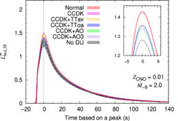
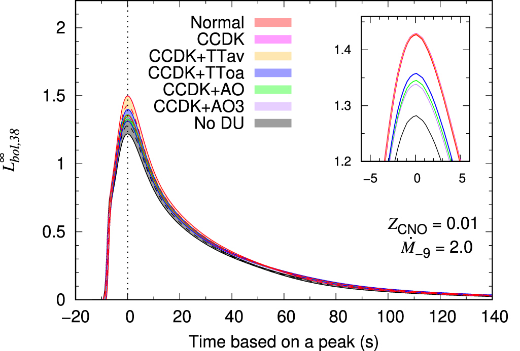
Simulated light curves during an X-ray burst, showing the effects of incorporating different physics. A model without neutrino cooling (labeled “No DU” in reference to the neutrino cooling pathway called direct Urca), peaks at a lower luminosity than models incorporating neutrino cooling. [Adapted from Dohi et al. 2022]

Sometimes, neutron stars reveal themselves by interacting with other stars. When a neutron star gathers gas from a stellar companion, the gas can ignite on the star’s scorching surface, resulting in a sudden burst of X-rays. After this sudden influx of heat, how does the neutron star cool, and how is the cooling reflected in the star’s light curve? While this may seem like a simple question, the answer hinges on our understanding of the conditions within the neutron star’s interior as well as the characteristics of the gas being accreted.

In a recent publication, a team led by Akira Dohi (土肥明; Kyushu University, Japan) explored the issue of neutron star cooling with general relativistic stellar evolution models. Specifically, the team investigated the effects of cooling by emitting neutrinos — chargeless, nearly massless particles that scarcely interact with matter — which is expected to speed up the cooling rate. The authors found that neutrino cooling increases the time between outbursts but makes them brighter at their peak, though additional physics to be included in future modeling might suppress this effect.

demonstration of subpulse drifting in simulated pulses

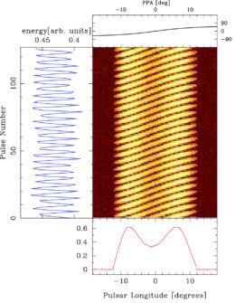
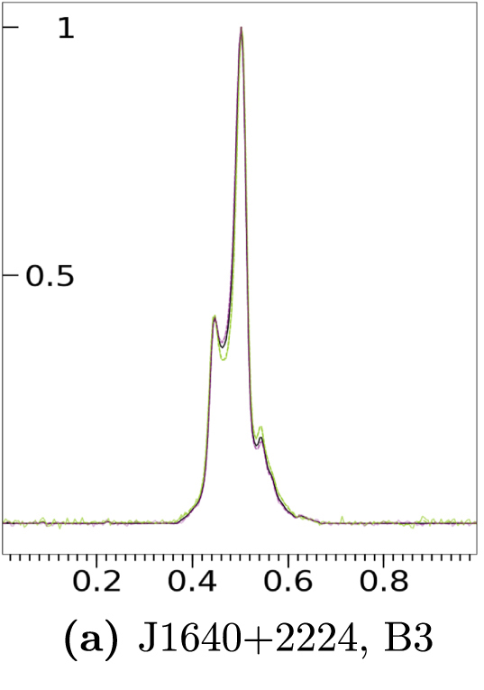
Simulated pulses showing a change in the phase of the pulse due to the shifting motion of the sparks. [Adapted from Basu et al. 2022]

Simulating Pulsar Sparks

Rahul Basu (University of Zielona Góra, Poland) and collaborators reported on simulations of conditions very close to the surface of a neutron star that emits beams of radio emission. Neutron stars that emit beamed radio waves are called pulsars for the way the beams sweep across our field of view, generating what we see as pulses of emission. Near a pulsar’s surface, extremely high temperatures and strong magnetic and electric fields combine forces to summon a sea of charged particles that are then accelerated to relativistic speeds.

Basu and collaborators focused on a phenomenon called sparking, in which charged particles jump the gap between the pulsar’s surface at its poles and its plasma-rich magnetosphere. The team’s modeling demonstrated that a pulsar’s poles are tightly filled with constant sparks, and the arrangement of these sparks slowly shifts over time. By modeling the emission associated with the simulated sparks, the team showed that the shifting motion of the sparks appears to be responsible for the observed periodic variations in the phases and amplitudes of some pulsars’ pulses.

Pulsars Probing Gravitational Waves

example of a pulsar radio pulse

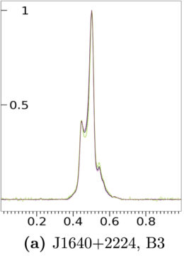
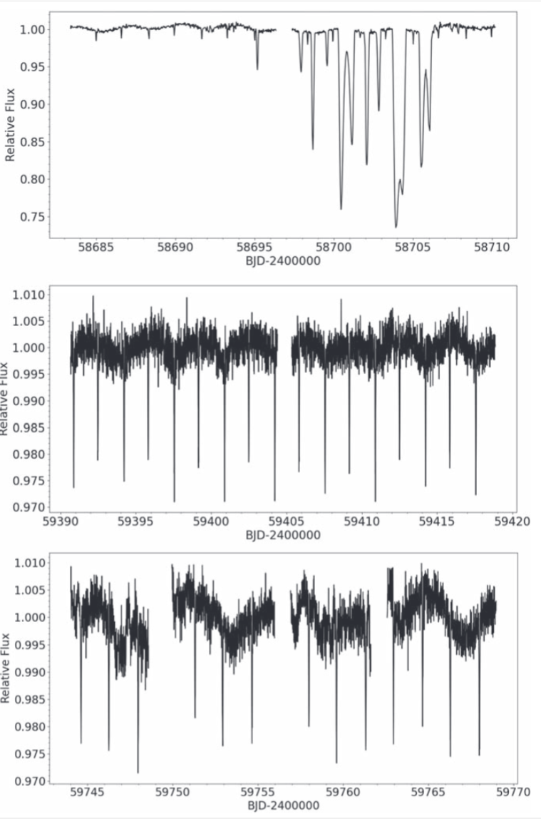
Example of a pulse observed with the Giant Metrewave Radio Telescope. [Adapted from Sharma et al. 2022]

By studying large groups of pulsars, astronomers hope to learn about something seemingly unrelated: gravitational waves. Pulsars provide a method to detect gravitational waves by way of these stars’ impeccable timekeeping abilities — because a pulsar’s radio beat is so reliable, the slight distortion of space caused by a passing gravitational wave should impact the arrival times of a pulsar’s pulses.

However, there’s a complication to this technique: spatial and temporal changes in the interstellar medium plasma can also affect when a pulsar’s radio pulses arrive at Earth. In order to compensate for the effect of the interstellar medium, we need to be able to make precise observations of pulsars across a range of radio frequencies. In a recent research article, Shyam Sharma (Tata Institute of Fundamental Research, India) and collaborators tested a pulsar-timing measurement technique using the Giant Metrewave Radio Telescope, which is highly sensitive to low-frequency radio waves. Sharma and coauthors showed that observing using a wide frequency band yields results comparable to typical narrowband observations, indicating that this technique could be used to disentangle the effects of the interstellar medium and more accurately time the pulses of arrays of pulsars, opening a new window onto gravitational waves.

simulated magnetar temperature maps

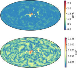
Temperature maps of the top of a magnetar’s crust (top) and the magnetar’s surface (bottom) after a hotspot is injected. [De Grandis et al. 2022]

Magnetic Outbursts

As if neutron stars could get any wilder: some neutron stars, dubbed magnetars, have extremely strong magnetic fields and exhibit frequent X-ray flares. While the cause of these X-ray outbursts is still unknown, some researchers have suggested that they arise from a sudden upwelling of magnetic energy beneath the magnetar’s crust, creating a hot spot that cools gradually over days or months.

To understand how the injection of heat into a magnetar’s crust might create the spectral features seen during X-ray outbursts, Davide De Grandis (University of Padova, Italy) and coauthors employed a three-dimensional magnetothermal model of hotspot formation and cooling. This model allowed the team to study the effects of asymmetrical hot spots under a magnetar’s crust for the first time. The team was able to confirm that these hot spots can be responsible for outbursts, though we’ll have to wait for future research to fully explore the evolution of the spectral features generated during these events.

Citation

“Impacts of the Direct Urca and Superfluidity inside a Neutron Star on Type I X-Ray Bursts and X-Ray Superbursts,” A. Dohi et al 2022 ApJ 937 124. doi:10.3847/1538-4357/ac8dfe

“Two-dimensional Configuration and Temporal Evolution of Spark Discharges in Pulsars,” Rahul Basu et al 2022 ApJ 936 35. doi:10.3847/1538-4357/ac8479

“Wide-band Timing of GMRT-discovered Millisecond Pulsars,” Shyam S. Sharma et al 2022 ApJ 936 86. doi:10.3847/1538-4357/ac86d8

“Three-dimensional Magnetothermal Simulations of Magnetar Outbursts,” Davide De Grandis et al 2022 ApJ 936 99. doi:10.3847/1538-4357/ac8797

A image of a globular cluster taken by the Hubble Space Telescope.

There are light curves, then there are light curves. Recently, astronomers untangled a particularly complex signal and revealed its surprisingly elegant cause: not one, two, or even three, but four stars locked into a never-ending dance.

A Mystery Light Curve

Over the past 20 years, astronomers have piled up quite the hoard of stellar light curves. Most of these are predictable, fairly simple time series: sure, the brightness of a given star might oscillate pseudo-regularly around its average as star spots come and go or the star shrinks and swells, but by and large, most curves don’t reveal anything surprising. A handful of exciting curves shelter the telltale signature of a transiting planet. Another handful hosts the unfortunately similar signature of eclipsing binary stars. Almost all of them can be explained by fairly simple models, just one or two stars and their planets going about their usual lives.

A three panel plot, each of which show brightness over time. In the top panel, the brightness changes dramatically and seemingly randomly, but in the lower two it oscillates regularly with a small amplitude

Measurements of TIC 114936199’s brightness over time, as observed in three different TESS sectors. Note the changes to the y-axis scale after the first sector. [Powell et al. 2022]

However, a few light curves among the hundreds of thousands recorded so far are bafflingly weird. Take the measurements of the source named TIC 114936199, which the Transiting Exoplanet Survey Satellite (TESS) watched in three disconnected chunks of about 30 days.

The second and third of these chunks look like a standard eclipsing binary. But that first stare… What could cause such deep, non-repeating dips?

To find out, a team led by Brian Powell (NASA Goddard Space Flight Center) started looking into arrangements of more and more eclipsing stars to explain how nature could create such strange dips in the first sector but not the others. A few clues led them to consider assemblages of four stars, which had been spotted by TESS before. But actually describing the size, location, and velocities of those four stars proved quite the challenge.

Fitting Challenges

A top-down schematic of the star system. Stars are represented as dots, and their motion is denoted by arrows. Stars Aa and Ab circle each other, star B circles the A pair, and star C circles the inner three.

A cartoon illustration of TIC 114936199’s components: four stars all bound together. The deep eclipses were the result of stars Aa and Ab passing in front of star C at the same time. [Powell et al. 2022]


Wandering the landscape of such a broad parameter space, Powell and collaborators found that standard Monte Carlo fitting routines got lost in the hills of local minima and could not find a reasonable solution. The team first increased their computational firepower by switching to a NASA supercomputer, then they deployed other algorithms such as Particle Swarm Optimization and Differential Evolution. In this exploration phase, the team churned through millions of possible combinations over many hundreds of thousands of computing hours.

All of this effort got them within the ballpark of a reasonable solution, and when they sensed they were close, the team again unleashed their fitting algorithm. This time, it made a beeline for their final solution, a configuration of four stars circling three different centers.

Successful Solution

A plot showing brightness over time of the first TESS sector. The data is shown as blue dots, and the final model is shown as a red line. The model faithfully follows each of the many dips in the data.

A zoom-in of data from the first TESS sector (blue) compared with the final model (red line). The residuals are shown below the time series. [Powell et al. 2022]

The model precisely predicted every one of the many dips in the intricate pattern in the first TESS sector, and it successfully explained why the pattern did not repeat: the innermost stars, Aa and Ab, eclipse each other every 3 days, but for 12 days in that first sector, they both also occasionally eclipsed star C as it drifted through the background. That particular arrangement should happen again in 2025, but after that we’ll have to wait much longer for the next lineup in 2071. While this isn’t the first quadruple star system observed by TESS, it is the first in this 2+1+1 configuration. Hopefully, astronomers will be able to observe the next series of complex eclipses in three years’ time — if not, they’ll have to wait a half century before enjoying such a dramatic show again.

Citation

“TIC 114936199: A Quadruple Star System with a 12 Day Outer-orbit Eclipse,” Brian P. Powell et al 2022 ApJ. 938 133 doi:10.3847/1538-4357/ac8934

Artist's impression of a young planetary system

A recent study suggests that protoplanetary disks may tend to linger longer than we thought, meaning that planets likely have at least 5 million years to form before their building materials vanish.

Disk Dispersal Deadlines

illustration of a protoplanetary disk being evaporated by a nearby massive star

One way that protoplanetary disks are dispersed is by radiation and winds from massive stars, as shown in this illustration. [NASA/JPL-Caltech]

Planets arise from gaseous disks called protoplanetary disks. While the details of planet formation are hidden from view within these dusty disks, the big picture is clear: the timeline for planet formation is set by the lifetime of the disk — once the disk disperses, planet formation must come to a halt. Determining how long planets have to form should be a simple task, then: researchers can measure the ages of star clusters and determine whether the stars in those clusters have disks, thus establishing a cutoff point at which disks typically disperse.

In reality, however, this technique has produced a wide range of estimates for the lifetimes of protoplanetary disks, and thus widely varying constraints on how long planets have to form — and the shortest estimates, in the 1.0–3.5 million year range, set a tight deadline for models of planet formation to meet.

Plot of disk fraction as a function of cluster age and distance

Fraction of stars with disks as a function of cluster age and distance. More distant clusters tend to have smaller disk fractions. [Adapted from Pfalzner et al. 2022]

Young, Massive, and Misleading?

In a recent publication, a team led by Susanne Pfalzner (Jülich Supercomputing Center and Max Planck Institute for Radio Astronomy, Germany) suggested that careful application of existing techniques can provide a little more wiggle room for modelers, lengthening the typical lifetime of a protoplanetary disk. Researchers often study disks around stars in clusters, since it’s more straightforward to determine their ages than stars outside of clusters. However, it’s easier to identify young, compact clusters than it is to find old, dispersed clusters, especially at large distances from Earth. Since bright, massive stars are easier to detect at large distances, studies biased toward younger clusters are also biased toward more massive stars — which are known to have shorter-lived disks.

As a demonstration of this effect, Pfalzner and coauthors examined how the results of previous studies varied with the properties of the clusters in each study’s sample. They found that samples containing mostly distant (>650 light-years away), young clusters resulted in short estimates for disk lifetimes, while samples containing nearby, old clusters were linked to long disk lifetimes.

Modelers Everywhere Breathe a Sigh of Relief

Plot showing the effect of stellar mass and initial disk fraction on the median disk lifetime in star clusters

The effect of stellar mass and initial disk fraction (IDF) on the median disk lifetime in star clusters. [Adapted from Pfalzner et al. 2022]

To counteract this issue, the team constructed a new sample that is evenly balanced between young and old clusters that are located within 650 light-years of Earth. Analysis of this sample suggested a median disk lifetime of 6.5 million years, with a substantial fraction of disks enduring for 10–20 million years — meaning that in many star systems, planets have far longer to form than expected.

While this result provides much-needed leeway for our models of planet formation, there are still plenty of open questions to explore. For example, it’s important to pin down the fraction of stars that are born with disks; assuming that all stars are initially shrouded in disks implies typical disk lifetimes in the 5–6 million year range, while allowing for a small fraction of stars to be born diskless would allow planets 8–10 million years to form around low-mass stars and 4–5 million years to form around high-mass stars. Regardless of the exact timeframe, understanding how high-mass stars form planets under stricter timescales than low-mass stars will remain a challenging question to answer.

Citation

“Most Planets Might Have More than 5 Myr of Time to Form,” Susanne Pfalzner et al 2022 ApJL 939 L10. doi:10.3847/2041-8213/ac9839

multiwavelength image of the galactic center region

The massive young stars at the center of the Milky Way have long puzzled astronomers. Did these stars form in a supermassive black hole’s backyard, or did they travel to the galactic center after their birth? In a recent publication, researchers proposed an entirely new scenario, in which the demise of one star prompts the formation of many more.

Born in a Black Hole’s Shadow

diagrams indicating the locations of stars within the disks

Locations of stars belonging to the putative clockwise and counter-clockwise disks at the center of the Milky Way. Distances are given in arcseconds. Click to enlarge. [Paumard et al. 2006]

At the center of our galaxy, massive young stars trace tight orbits around a supermassive black hole. When researchers charted these stars’ paths, a curious pattern emerged: several dozen stars were arrayed in one or more narrow disks that are off kilter from the plane of the galaxy.

The presence of young stars in the hostile inner regions of our galaxy is mysterious enough, and this arrangement is even more perplexing. It’s not yet clear how stars might form so close to a black hole — the tidal forces should prevent new stars from coalescing — and the disk-like arrangement shouldn’t arise naturally if the stars migrated from elsewhere in the galaxy. How did these stars come to be where they are?

diagram of the authors' jet–cocoon system

Diagram of the jet–cocoon configuration. Because the pressure within the cocoon exceeds the pressure of the surrounding gas clouds, the cocoon sweeps outward and compresses the clouds nearby. [Perna & Evgeni 2022]

From Disruption to Disk Formation

Rosalba Perna (Stony Brook University and Flatiron Institute) and Evgeni Grishin (Monash University and Australian Research Council Centre of Excellence for Gravitational Wave Discovery) proposed that when a star is tidally disrupted by a supermassive black hole, it creates the conditions for new stars to form.

Here’s how it works: in rare cases, as a star is being pulled apart by a black hole, it shoots out a jet of material. A cocoon of gas enclosing this jet expands perpendicular to the jet, compressing the surrounding gas and providing enough pressure for gas clumps to overcome the black hole’s tidal pull and form new stars.

While the expanding cocoon spurs star formation perpendicular to the jet, the jet itself creates a cone of superheated gas that suppresses star formation along its length. The combination of these factors promotes star formation in a thin disk, and the orientation of the disk is linked to the orbit of the disrupted star. In other words, the team expects that a tidally disrupted star will lead to a disk of stars forming at a random angle with respect to the galactic plane — exactly the arrangement we see at the center of the Milky Way.

More to Learn

The Milky Way’s supermassive black hole likely tidally disrupts a star once every 10,000–100,000 years, with jetted tidal disruption events occurring every 1–10 million years. Why, then, have we only found evidence for two misaligned disks of stars at the galactic center? Because this method tends to form massive stars, the disks should disappear quickly; stars formed in the wake of a tidal disruption event would survive only a few million years.

While this scenario laid out by Perna and Grishin appears to answer many of the questions regarding the stars arrayed in disks near the center of the Milky Way, the authors acknowledged that their hypothesis needs to be tested thoroughly. Hopefully, future numerical simulations will help us close in on the formation mechanism for these galactic center stars!

Citation

“Disks of Stars in the Galactic Center Triggered by Tidal Disruption Events,” Rosalba Perna and Evgeni Grishin 2022 ApJL 939 L17. doi:10.3847/2041-8213/ac99d8

An artist's impression of an X-ray burst

When a neutron star snares material from a stellar companion, we see a flash of X-rays called an X-ray burst. What can an analysis of 51 bursts from a single source tell us about the physics behind these events?

Bursting Binary Systems

photograph of the NICER telescope on the International Space Station

A view of the Neutron star Interior Composition Explorer (NICER), seen at the center of this image, in its berth on the International Space Station. [NASA]

Binary systems containing a neutron star — the extremely dense core of an expired massive star — and a main-sequence, supergiant, or white dwarf star are called X-ray binaries for the short bursts of X-rays they emit. These outbursts are thought to arise when the neutron star accretes gas from its stellar companion, forming an accretion disk from which the neutron star siphons a stream of material that ignites in a brief flash of nuclear fusion. Studying X-ray bursts allows researchers to pin down the properties of neutron stars and understand the physics that governs accreted gas.

One of our best tools for studying these bursts is the Neutron star Interior Composition Explorer (NICER), which has monitored X-rays from its vantage point on the International Space Station since 2017. Among NICER’s many targets is the highly active binary 4U 1636–536, which was discovered just over 50 years ago. Researchers have cataloged hundreds of X-ray bursts from 4U 1636–536, finding that it averages one burst every four hours!

example of an X-ray burst

An example of an X-ray burst from 4U 1636–536 as seen by NICER. [Adapted from Güver et al. 2022]

Accretion Increases and Disk Reflections

In a recent publication, a team led by Tolga Güver (Istanbul University) searched for evidence of additional X-ray bursts from 4U 1636–536 during a monitoring campaign with NICER. Güver and collaborators identified 51 X-ray bursts during 138 observations and collected spectra for 40 of them, allowing the team to characterize 4U 1636–536’s bursting behavior and understand how X-ray bursts affect their surroundings.

Güver and collaborators found that all of the bursts for which they acquired spectra had an excess of soft (i.e., low-energy) X-ray emission. Modeling of this spectral feature indicated that it likely arises from either an increase in the rate at which matter is accreted onto the neutron star or from the burst scattering off the disk and/or being absorbed and re-emitted at a different wavelength, a process referred to as reflection. However, many of the bursts were fit well by models of both scenarios, and the authors pointed out that both processes likely occur simultaneously.

Further X-ray Investigations

To learn even more about 4U 1636–536’s frequent outbursts, Güver and collaborators analyzed data from India’s multi-wavelength space telescope AstroSat and the Nuclear Spectroscopic Telescope Array (NuSTAR). Using NuSTAR data, the team searched for evidence of Compton cooling, in which high-energy photons lose some of their energy through collisions with nearby electrons. The team discovered decreases in the hard (i.e., high-energy) X-ray emission shortly after the onset of several bursts, but the low count rate prevented a firm detection.

chi-squared distributions for the two models tested on the NICER data

Comparison of reduced χ2 values for best fits to the NICER spectra using the disk reflection model (blue) and the increased accretion model (red). [Güver et al. 2022]

The authors also used observations of several bursts made by AstroSat and NuSTAR to probe the causes of the excess soft X-ray emission further. Similar to their investigations of the NICER spectra, the team found that they could fit the spectra with either a disk reflection model or an increased accretion model — but simultaneously modeling both of these effects will require brighter X-ray bursts or a larger telescope.

Citation

“Burst–Disk Interaction in 4U 1636–536 as Observed by NICER,” Tolga Güver et al 2022 ApJ 935 154. doi:10.3847/1538-4357/ac8106

1 30 31 32 33 34 112