Astrobites RSS

brown dwarf

Editor’s note: Astrobites is a graduate-student-run organization that digests astrophysical literature for undergraduate students. As part of the partnership between the AAS and astrobites, we occasionally repost astrobites content here at AAS Nova. We hope you enjoy this post from astrobites; the original can be viewed at astrobites.org.

Title: Direct radio discovery of a cold brown dwarf
Authors: H. K. Vedantham et al.
First Author’s Institution: ASTRON, Netherlands Institute for Radio Astronomy
Status: Submitted to ApJL

Brown Dwarfs: The Middle School of Celestial Objects

What do you get when you have too much mass to form a planet, but not enough mass to form a star? A brown dwarf! First theorized in the 1960s and observed in the 1990s, brown dwarfs — a subclass of ultra-cool dwarfs — are substellar objects around 13–80 times the mass of Jupiter (or 10–90 times, depending on who you ask). They are special because, though they are thought to form in a similar manner to stars, they aren’t massive enough to trigger sustained hydrogen fusion in their cores. Instead, they are thought to fuse deuterium or lithium. This means that, unlike our Sun or other stars, they will gradually cool and fade rather than becoming white dwarfs, neutron stars, or black holes.

Despite not being stars, brown dwarfs are still self-luminous — meaning they emit energy in the form of light rather than just reflecting it back from a host star — and therefore can have spectral classifications like stars. Depending on how much light they emit and their temperatures, brown dwarfs are classified as either L, T, or Y type. Each class shows different dominant absorption lines: L dwarfs are water- and carbon-monoxide-dominated, T dwarfs are methane-dominated, and Y dwarfs are potentially ammonia-dominated.

The Study

Like stars, some brown dwarfs are known to have strong magnetic fields, and even instances of potential aurorae. In addition to being observable by some optical instruments, this magnetic activity allows some brown dwarfs to be detectable in the radio and — if the magnetic field activity is strong enough — X-ray bands. However, radio observations of these objects have previously been performed primarily to follow-up known brown dwarfs. The authors of today’s paper use the Low Frequency Array (LOFAR) to make the first direct radio discovery of a brown dwarf, BDR 1750+3809. They specifically looked at circularly polarized radio sources in the LOFAR Two-meter Sky Survey (LoTSS), because known brown dwarfs have highly circularly polarized radio emission. They followed up the LoTSS data with near-infrared observations using the Wide-field Infrared Camera (WIRC) at Palomar, and the NIRI imager at Gemini-North. They also obtained a spectrum using NASA’s Infrared Telescope Facility (IRTF).

Using all of these follow-up observations, the authors were able to determine several characteristics of BDR 1750+3809:

  • It has strong methane absorption bands, indicating it is likely a T dwarf
  • The approximate distance to the object, calculated using the distance modulus, is around 57–74 pc (186–241 light-years)
  • It has a larger luminosity than expected. This is likely caused by the viewing geometry or by a companion object that is either large or close to BDR 1750+3809, similar to the Jupiter–Io system.

Most importantly, though, the detection shows that radio observations can be used to blindly discover these objects.

LOFAR observations

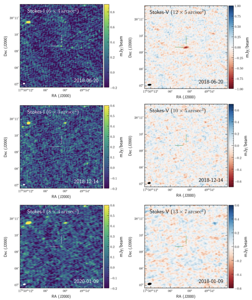
Figure 1: Six graphs of LOFAR radio signals (and non-detections) from BDR 1750+3809 are shown. The graphs on the left show the total intensity of the signal, while the graphs on the right show only the intensity of the circularly polarized signals. The three different observation dates are noted on the graphs. [Vedantham et al. 2020]

Why Does It Matter?

This discovery is important not only as evidence of a way to discover more brown dwarfs, but also as a potential window into learning more about the properties of exoplanet magnetospheres. Both brown dwarfs and planets are thought to have exclusively dipolar magnetic fields, meaning they have two poles of equal and opposite strength like a bar magnet or Earth’s magnetic field. However, because of technological constraints and the fact that Earth’s ionosphere blocks many low-frequency radio waves, signals from exoplanet magnetic fields are currently hard to detect (although one was detected via its aurorae earlier this year). This low-frequency brown dwarf observation — comparable to what is expected from gas giant exoplanets — indicates that instruments such as LOFAR do have the sensitivity necessary to make radio detections of exoplanet magnetospheres. If learning about the magnetic field itself isn’t exciting enough, keep in mind that a magnetic field strong enough to shield a planet from stellar radiation is a requirement for habitability as we know it. The more we can determine about an exoplanet’s magnetosphere, the more we can speculate about the possibility of it sustaining life!

Original astrobite edited by Aaron Pearlman.

About the author, Ali Crisp:

I’m a third year grad student at Louisiana State University. I study hot Jupiter exoplanets in the galactic bulge. I am originally from Tennessee and attended undergrad at Christian Brothers University, where I studied physics and history. In my “free time,” I enjoy cooking, hiking, and photography.

circumbinary transit

Editor’s note: Astrobites is a graduate-student-run organization that digests astrophysical literature for undergraduate students. As part of the partnership between the AAS and astrobites, we occasionally repost astrobites content here at AAS Nova. We hope you enjoy this post from astrobites; the original can be viewed at astrobites.org.

Title: Hidden Worlds: Dynamical Architecture Predictions of Undetected Planets in Multi-planet Systems and Applications to TESS Systems
Authors: Jeremy Dietrich and Dániel Apai
First Author’s Institution: The University of Arizona, Tucson
Status: Published in AJ

Fans and writers of science fiction alike spend countless hours crafting intricate star systems, replete with planets, moons, and a menagerie of space-faring civilisations. The success of missions such as the Kepler Space Telescope (hereafter Kepler) and the Transiting Exoplanet Survey Satellite (TESS) have shown that our solar system is just one of many multi-planet systems present throughout the Milky Way. However, our ability to accurately determine the “planetary architecture” (the orbital configuration of the planets) of a given extrasolar system is severely lacking. Knowing how planets are configured in different extrasolar systems would greatly aid our understanding of how planets form, and how planetary systems evolve (e.g., via planetary migration).

Exoplanets are inherently difficult to detect, and one of the primary means of detecting them involves measuring transits, the tiny dimming of a star as a planet moves in front of it. To better understand stellar systems, instead of considering each exoplanet individually, we can consider the entire population of exoplanets at once through statistical inference — a method that has only recently become viable thanks to the wealth of data from modern exoplanet surveys. Today’s paper presents a statistical framework — DYNAmical Multi-planet Injection TEster (DYNAMITE) — designed to predict the presence of exoplanets that have so far eluded detection.

Fire in the Hole!

The core method at the heart of DYNAMITE is to determine the likelihood of finding an additional planet in an existing multi-planet system, based on the overall statistics of an existing representative population. The authors consider a combined probability density function (PDF) over the inclination, orbital period, and planetary radius, with the key assumption being that each of these parameters has its own independent distribution. Each of these initial PDFs were based on transiting planet data from Kepler, with the range of orbital periods restricted from 0.5 to 730 days, planetary radii from 0.5 to 5 Earth radii, and inclinations between 0 and 180 degrees. Monte Carlo methods (means of approximating something through repeated random sampling) are then used to sample the full probability distributions and “inject” new planets into the system. In order to come up with sensible results, the planetary system must be dynamically stable. This stability depends on the orbits of the innermost and outermost planets, their masses, and the mass of the parent star. It is difficult to accurately determine the masses of exoplanets via the common transit method, so the authors make use of a mass–radius relation to estimate the masses from the planetary radii.

Sweet Spot

Kepler-154 system

Figure 1: The probability distribution function for the Kepler-154 system with the 9.92-day-period planet removed (outlined cross). Blue spikes indicate individual Monte Carlo injections. Green circles indicate the relative sizes of the known planets. Click to enlarge. [Dietrich & Apai 2020]

The model underwent rigorous testing for sensitivity and robustness. Several test scenarios included removing a known planet to see if the model could reproduce it, and removing a planet whilst altering the remaining planets. Figure 1 shows an example of the PDF as a function of orbital period for the Kepler-154 system with the known planet at P = 9.92 days (Kepler-154 f) removed. Of the total Monte Carlo predictions that inject a new planet inside the orbit of the outermost planet, 97% correspond to the region of the removed planet. As for the radius, 67% of the models predictions lie within three standard errors, while the spread is more substantial for the inclination (43%). The mean injections match the known planet’s parameters quite well (as in Figure 1 where the peak is just below the known value for the period), but the authors nevertheless state that since DYNAMITE is primarily aimed at helping guide future observations, it is not designed to provide exact predictions, but rather a likely range of values.

Speculative Execution

One of DYNAMITE’s major applications lies in the analysis of systems with candidate planets — planets that are suspected to be there but have not yet been definitively confirmed. TOI 1469 is used as an example to illustrate the iterative nature of the statistical model. Figure 2 shows the various stages of DYNAMITE for the TOI 1469 (HD 219134 / Gliese 892) system. This system is known to have two transiting planets, with at least three non-transiting planets. Starting with only the two known transiting planets, the PDF peaks at around 12.5 days. A planet is inserted here, and the model is run again. Now the PDF peaks near the known planet at around 23 days (HD 219134 f has a period of 22.72 +/- 0.02 days), so we insert another planet here and execute the model again. Proceeding in this manner, the model predicts another planet at ~46 days (corresponding to HD 219134 f with orbital period 46.86 +/- 0.03 days), while in the last iteration the model predicts a fourth planet at ~87 days, corresponding to the unconfirmed candidate planet.

TOI 1469 multi-planet system

Figure 2: Probability distribution functions of the orbital period for each iteration of DYNAMITE for the TOI 1469 multi-planet system. [Dietrich & Apai 2020]

To Probability Space and Beyond

predicted planet period-radius likelihoods

Figure 3: 2D normalised probability densities in log radius and log period. Brighter regions correspond to a higher probability of a predicted planet. Multi-planetary systems are marked along with their TESS TOI identifiers. Ellipses indicate one standard error. [Dietrich & Apai 2020]

Another purpose of DYNAMITE is to analyse the newly identified multi-stellar systems discovered by TESS and identify the systems most likely to contain additional planets so that they can be surveyed again. A sample of known multi-stellar systems from the ExoFOP-TESS archive was tested with the statistical model. Figure 3 shows the overall results of the model using the period ratio model from Kepler, while Figure 4 shows the exact PDF for each TESS system for the orbital period and planetary radius.

With the ability to predict the locations of hitherto undetected planets, future surveys can be more focused and targeted. Studying these systems in detail, and confirming whether or not these additional planets are present, allows us to constrain and refine models of planetary architectures, our knowledge of the mechanisms that govern the evolution of planetary systems, and, ultimately, our understanding of how exoplanets form.

normalized PDF for TESS systems

Figure 4: The normalised PDF for each TESS sample for orbital period (left) and planetary radius (right). Red dots indicate known planets, with the size of each dot representing that planet’s relative size. Darker regions highlight the most likely regions in which to find additional planets. [Adapted from Dietrich & Apai 2020]

About the author, Mitchell Cavanagh:

Mitchell is a PhD student in astrophysics at the University of Western Australia. His research is focused on the applications of machine learning to the study of galaxy formation and evolution. Outside of research, he is an avid bookworm and enjoys gaming, languages, and code jams.

protocluster

Editor’s note: Astrobites is a graduate-student-run organization that digests astrophysical literature for undergraduate students. As part of the partnership between the AAS and astrobites, we occasionally repost astrobites content here at AAS Nova. We hope you enjoy this post from astrobites; the original can be viewed at astrobites.org.

Title: Emergence of an Ultra-Red, Ultra-Massive Galaxy Cluster Core at z = 4
Authors: Arianna S. Long et al.
First Author’s Institution: UC Irvine
Status: Published in ApJ

Galaxy clusters are vast entities. They contain 100 to 1,000 galaxies, making them the largest gravitationally stable structures in the cosmos. One of the assumptions of our understanding of the universe is that structures form hierarchically — smaller gravitational objects form first, followed by the largest. Therefore, to form large objects like clusters, smaller objects such as galaxies need to collide and merge together over a long period of time.

Although we generally know how clusters form, the specific process by which they grow is not yet well understood. The progenitors of clusters, known as protoclusters, are typically found at redshifts greater than z = 2 (the higher the redshift, the farther back it is in time), when the universe was about one third of its current size. Unlike the clusters we observe today, protoclusters do not appear to have an established population of “red and dead” elliptical galaxies, which makes them harder to identify. Instead, protoclusters are usually identified by overdensities of star forming galaxies known as Lyman-alpha emitters, which are typically studied using data in the optical and ultraviolet (UV) wavelength ranges. You can check out other Astrobites on the intriguing properties of protoclusters here, here, and here.

The Hunt for Protoclusters

Today’s paper offers an alternative method for identifying protoclusters via a certain galaxy population known as dusty star forming galaxies (DSFGs). These galaxies contain substantial amounts of dust, which obscures their optical/UV light, but allows them to glow in infrared (IR). DSFGs are capable of forming stars in a short period of time at higher redshifts, which allows them to become the large red elliptical galaxies we see in clusters later on. DSFGs are also typically found in the vicinity of other DSFGs, which suggests they are pivotal to protocluster evolution.

Although protoclusters with DSFGs have been observed before, these have almost all been at redshifts below z = 3. Above this, a handful of protoclusters have been found, but studies are considerably more limited in resolution and the ability to spectrally classify such galaxies.

The authors of today’s paper present insights into the gas, dust, and stellar properties within a distant (z = 4!) protocluster containing 11 tightly bound DSFGs, known as the Distant Red Core (DRC). For the first time, this system has new high resolution HST (optical) and Spitzer (infrared) observations, bolstered with existing ALMA (submillimetre), Gemini (near infrared), and Herschel (far infrared/submillimetre) data.

Different components of the protocluster are shown in Figure 1 using the Spitzer, Gemini and HST data. Combining multiwavelength data is crucial to ensuring that the DRC and potential other members comprise a genuine physical system, and to bypass issues where two or more galaxies appear as one in an image due to blending effects. Within some of these, we can see evidence of merging (e.g., in the long elliptical structure of DRC8). The authors note that although there are 11 in total, only 10 are spectroscopically confirmed to be at z = 4 (all except DRC 5).

protocluster

Figure 1: The Spitzer data highlights the protocluster core within the green box in the leftmost image, while the pink circles labeled C–G show the positions of other potential protocluster members. The Gemini image (middle) zooms in on the protocluster core, with each of the 10 components circled in green. The HST image on the right confirms the appearance of 11 DRC components. [Long et al. 2020]

Outstanding in the Field?

Each of the galaxies in the DRC have approximately similar masses (>1010 solar masses). Interestingly, they exhibit minimal differences in star formation rate and mass when compared with other galaxies at z ~ 4 that aren’t in clusters (known as the “field”). The authors demonstrate that the DRC members fit neatly within one standard deviation of the measured main sequence (MS) relation at z = 4 (shown in Figure 2). Previous studies have also expected to find more gas in galaxies in cluster environments compared to field galaxies, but the results do not confirm this.

star formation rates

Figure 2: Star formation rate of galaxies from various studies, including the DRC objects, as a function of their stellar mass. The majority of DRC objects (given by the circled numbers) are shown to be within the bounds of the main sequence (MS) relation. This broadly agrees with galaxy populations from various other studies. [Long et al. 2020]

Weighing It Up

Finally, the authors infer the total mass of the protocluster. This is difficult, as it includes not just the individual stars in galaxies, but the underlying dark matter distribution encompassed within the cluster halo. As we cannot see dark matter, some assumptions are required to determine the total mass. Fortunately, a well-known relationship exists between the stellar and total mass of galaxies, assuming stars in galaxies accurately trace the dark matter content. By summing the masses of the individual galaxy halos, and correcting to avoid double counting halos that overlap, the protocluster mass can be computed. As shown in Figure 3, the DRC is already at least as massive as protoclusters between redshifts of = 2 and = 3. Based on this data, the DRC is on course to evolve to above 1015 solar masses by the present day, which would make it one of the largest clusters in our cosmos.

halo mass v. redshift

Figure 3: Estimated total mass of the DRC using three different methods (purple dotted lines) compared to bounds on the allowed mass of protoclusters (red stars) over a range of redshifts. The DRC is at the same mass scale as a population of known protoclusters despite being considerably farther away. For comparison, the grey band shows the estimated growth for a Coma-like cluster over time. [Long et al. 2020]

Our current model of hierarchical structure formation allows us to predict the maximum possible mass of protoclusters at various times. The authors show the DRC is large enough that it is on the boundary of being excluded by our accepted cosmological model. Further observations of the DRC will be able to tell us whether such a massive protocluster really is causing a problem (it wouldn’t be the first time). The emergence of the DRC at z = 4 shines a new light on early cluster formation, while also leaving room for many exciting questions that will hopefully be answered in future protocluster studies.

About the author, Sunayana Bhargava:

I’m a 4th year PhD student at the University of Sussex, interested in X-ray and optical observations of galaxy clusters to learn more about dark matter and large-scale structure. When I’m not working, I’m usually trying to write in coffee shops or hiking.

perseus cluster gas

Editor’s note: Astrobites is a graduate-student-run organization that digests astrophysical literature for undergraduate students. As part of the partnership between the AAS and astrobites, we occasionally repost astrobites content here at AAS Nova. We hope you enjoy this post from astrobites; the original can be viewed at astrobites.org.

Title: A Novel Machine Approach to Disentangle Multi-Temperature Regions in Galaxy Clusters
Authors: Carter L. Rhea, et al.
First Author’s Institution: University of Montreal, Canada
Status: Accepted to AJ

Galaxy clusters are among the largest gravitationally bound structures in the universe. One of their defining characteristics is that they tend to be embedded within a large reservoir of superheated gas, known as the intracluster medium (ICM). With temperatures up to 10Kelvin, the ICM is a strong emitter of X-ray radiation. The resulting spectrum is dominated by thermal bremßtrahlung radiation: radiation emitted when charged particles are decelerated. Characterising this thermal emission provides useful insights into the physical processes within the cluster, such as galaxy merging and active galactic nucleus (AGN) activity, as well as various physical parameters including temperature and metallicity. In order to obtain these parameters, one must first fit the observed spectra. However, the ICM is not necessarily uniform. Different regions are often characterised by multiple thermal components, requiring a mix of temperatures rather than a single temperature model to reproduce the observed spectra. The authors of today’s bite propose a new machine-learning method to systematically estimate the different underlying thermal components in ICM spectra. As this approach is not reliant on any particular physical model, it is both efficient and portable.

The Component and The Forest

The authors’ machine-learning approach features two key techniques; principal component analysis (PCA) and random forests. The idea of PCA is to break large, multi-dimensional datasets into their principal components; these are a series of orthonormal basis vectors such that each vector points in a direction of maximal variance. This is analogous to solving for eigenvectors, and the data processing can be thought of as a change of basis. PCA is extremely useful for machine learning because it structures the data in a way that best highlights relevant features (while discarding those that are redundant/irrelevant). This improves the learning capability and efficiency of machine-learning techniques. The authors use a random forest of decision tree classifiers to classify the processed data (i.e. the data after having been transformed via PCA). In a decision tree, the dataset is recursively partitioned until each subset corresponds to a specific class or category. Since decision trees are quite unwieldy and prone to overfitting, it is often beneficial to train several thousand at once (i.e. a random forest). Given an input corresponding to a region of X-ray emission, the goal is to output the number of unique thermal components needed to describe the region. The authors create the training data using synthetic X-ray spectra based on observations taken from the Chandra observatory.

The King of Mycenae

The authors applied their machine-learning method to the Perseus cluster, which is known to have regions with multiple temperature components. Figure 1 shows that the overwhelming majority of the Perseus cluster consists of two-component thermal emission (blue), with some regions of four-component (yellow) and single-component (indigo) emission. This verifies previous conclusions, based on Chandra observations, that the Perseus cluster cannot be accurately modelled with a single temperature component.

perseus cluster temperature

Figure 1: A smoothed image of the X-ray emission from the Perseus cluster (left), compared to a Voronoi tessellation map of the predicted single component (indigo), double component (blue) and quadruple component (yellow) regions. There is a very small triple component (green) region in the brightest cluster galaxy (BCG). [Rhea, et al. 2020]

Mapping the Components

Having established that there are two main temperature components, the authors next calculated temperature maps. Figure 2 shows each of these components. Overall, each component corresponds to gases at different temperatures; the first component is characterised by a relatively cooler gas (of around 2 keV), while the second corresponds to a hotter gas (of 4 keV). These also correspond to soft and hard X-ray emission. What is encouraging is that these components are distributed differently: the cool gas is mostly uniform while the hot gas is more uneven. Some regions with a low first-component temperature have a high second-component temperature (and vice versa). Thus only by combining these different components can one accurately model the thermal nature of X-ray emission throughout the ICM.

temperature maps

Figure 2: Temperature maps (Voronoi) highlighting the first (left) and second (right) thermal components (for regions with exactly two components). Colour denotes the mean temperature of the gas. [Rhea, et al. 2020]

Onwards and Upwards

One of the major benefits of this machine-learning approach is that it is not solely restricted to Chandra data; it can be used with other X-ray missions such as Athena and eROSITA. The authors expect that future, high resolution surveys will result in improved classifications. This is since the random forest classification is sensitive to many factors including resolution, time epochs (since CCDs degrade over time), and selection biases in the choice of training data (e.g. redshift, column densities). The authors have demonstrated that a new machine-learning technique is capable of extracting the multiple thermal components in ICM X-ray emission, confirming that the Perseus cluster is indeed best characterised by more than one component. As future surveys yield stronger constraints on ICM emission, it will be possible to model physical processes in greater detail, ultimately improving our understanding of galaxy clusters and the evolution of galaxies contained within.

About the author, Mitchell Cavanagh:

Mitchell is a PhD student in astrophysics at the University of Western Australia. His research is focused on the applications of machine learning to the study of galaxy formation and evolution. Outside of research, he is an avid bookworm and enjoys gaming, languages, and code jams.

M dwarf planet

Editor’s note: Astrobites is a graduate-student-run organization that digests astrophysical literature for undergraduate students. As part of the partnership between the AAS and astrobites, we occasionally repost astrobites content here at AAS Nova. We hope you enjoy this post from astrobites; the original can be viewed at astrobites.org.

Title: The High-Energy Radiation Environment Around a 10 Gyr M Dwarf: Habitable at Last?
Authors: Kevin France, Girish Duvvuri, Hilary Egan, et al.
First Author’s Institution: University of Colorado Boulder
Status: Accepted to AJ

There are lots of stars out there in the universe, and a large chunk of those are M dwarfs. These are the smallest and reddest stars, coming last in the sequence of spectral types (O, B, A, F, G, K, and last but not least: M). Bonus: since they’re so small and dim, it’s actually easier to find smaller, terrestrial planets around them! Given that M dwarfs are so plentiful and we have a good shot at peering into their habitable zones, it makes sense that we’d want to think about what life on a planet around an M dwarf would be like.

flaring dwarf star

Artist’s rendering of a flaring dwarf star. [NASA’s Goddard SFC/S. Wiessinger]

But there’s a catch. M dwarfs are also known to be very active stars, flaring and giving off a lot of ultraviolet light and X-rays that are bad news for biological life. This stellar activity is so strong that it drives atmospheric escape, stripping these rocky planets of their atmospheres, which are critical for habitability. Extreme ultraviolet light (known as EUV or XUV) is particularly good at stripping away an atmosphere, and young M dwarfs give off more of this since they spend a longer time in their pre-main sequence evolution phase. So, the beginning of these stars’ lives are extreme, ruining chances for a planet to be habitable. What about older M dwarfs? Planets around M dwarfs could have a do-over on their atmosphere, gaining a “secondary atmosphere” created by gases released through impacts or volcanos. Do M dwarfs mellow with age, quieting down all that radiation and making it possible for their planets’ secondary atmospheres to stick around long enough for life to arise?

Today’s paper seeks to answer these questions by observing a nearby old M dwarf for its UV and X-ray activity, and then computing what would happen to the atmosphere of an Earth-like planet in its habitable zone.

The Search for the Atmosphere Killers

The authors used the Hubble Space Telescope (for UV observations) and the Chandra X-ray Observatory to observe Barnard’s Star, a nearby old M star. Barnard’s Star is only about six light-years away, making it one of our closest neighbors in space. It’s only 16% the size of the Sun, but about twice as old. It’s also known to host a cold (around –300°F!) super-Earth about three times the size of our planet, discovered using the radial velocity method.

The average UV luminosity of Barnard’s star is among the lowest ever measured for an M dwarf, but it still emits more XUV than the Sun, as shown in Figure 1. They also measured a weak (but non-zero) X-ray flux, also among the lowest observed on an M dwarf. Barnard’s Star still flared just about as frequently as younger M dwarfs, but the flares on the older star were lower intensity (still more intense than a star like our Sun, though!). Another atmosphere-harming event is the CME, or “coronal mass ejection”, which releases high energy particles from the star; the authors found that these events have similar energies to solar flares, but are much more frequent. There is a caveat on this, though: M dwarfs have been theorized to have stronger magnetic fields, which may keep CMEs from traveling far from the star and impacting planets, so there’s a bit of uncertainty on the effect of CMEs on an atmosphere discussed here.

sun v barnard

Figure 1: Sun (black) vs. Barnard’s star (red). Barnard’s star shows more extreme ultraviolet! [France et al. 2020]

The Verdict on the Atmosphere

Now that we know a bit more about the environment around an old M dwarf, what would happen to a planet’s atmosphere? The authors estimated the atmospheric escape from a hypothetical Earth-like planet in the habitable zone of Barnard’s Star that encounters this observed high-energy radiation.

First, to make sure their models made sense, they tested them on the Sun/Earth system to see if they could reproduce what we observe in our own solar system. Then, they moved on to look at the thermal and ion escape from our hypothetical planet. Thermal escape happens when particles are hot enough, and therefore moving fast enough, to exceed the escape velocity of the planet. Around Barnard’s Star, our hypothetical planet would lose its atmosphere in about 11 million years. Or, you can think about it as losing 87 times the Earth’s atmosphere in a billion years (for context, Earth is over 4 billion years old!).

They also looked at ion escape, which is actually the main way Earth loses atmosphere. This is a bit more complicated, since it requires a plasma interaction model. Their simulations showed that in a normal, quiescent (not flaring) state, Barnard’s Star only slightly increases atmospheric escape compared to Earth. However, when a flare happens, there is much more atmosphere loss, as seen in Figure 2. One thing to note is that the hypothetical planet here is unmagnetized; magnetism could make a difference, as it does on Earth, shielding from some of these high energy particles. The big takeaway here, though, is that atmospheric loss around old M dwarfs will be dominated by the flare periods.

ion loss

Figure 2: These simulations for show ion escape for three scenarios: base (unmagnetized Earth around the Sun), quiet (unmagnetized Earth-like planet in Barnard star habitable zone in quiescent conditions), and flare (same planet around Barnard star but during flare). The color bar corresponds to the amount of oxygen ions lost. [France et al. 2020]

Can Life Find a Way?

Flares might actually have a positive effect on life in a different way. Other work has shown that near-UV (NUV) photons might drive the formation of precursor molecules to RNA; Barnard’s Star has a little less NUV radiation than is needed for this in its quiet state, but flaring could be enough to support these prebiotic pathways. Also, now that we know flares might be an issue for keeping an atmosphere, we might want to extend our search for habitable planets out farther from the star; there’s a possibility of an “extended habitable zone” farther out from the star where the radiation is less extreme!

Although they’re less active, this paper has shown that even old M dwarfs can lose a lot of atmosphere, particularly due to flares. We still need to learn more about the flare cycles, since that seems to be a key parameter in atmospheric retention and M dwarf habitability!

About the author, Briley Lewis:

Briley Lewis is a second-year graduate student and NSF Fellow at the University of California, Los Angeles studying Astronomy & Astrophysics. Her research interests are primarily in planetary systems – both exoplanets and objects in our own solar system, how they form, and how we can create instruments to learn more about them. She has previously pursued her research at the American Museum of Natural History in NYC, and also at Space Telescope Science Institute in Baltimore, MD. Outside of research, she is passionate about teaching and public outreach, and spends her free time bringing together her love of science with her loves of crafting and writing.

AGN illustration

Editor’s note: Astrobites is a graduate-student-run organization that digests astrophysical literature for undergraduate students. As part of the partnership between the AAS and astrobites, we occasionally repost astrobites content here at AAS Nova. We hope you enjoy this post from astrobites; the original can be viewed at astrobites.org.

Note: the title of this article has been changed from its original version.

Title: The Role of Active Galactic Nuclei in the Quenching of Massive Galaxies in the SQuIGGLE Survey
Authors: Jenny E. Greene et al.
First Author’s Institution: Princeton University
Status: Published in ApJL

To butcher an apocryphal quote about cars, galaxies can be any colour, as long as it’s red or blue. If you were to plot the magnitude and colour of a large sample of galaxies you would see that they fall into two groups: one is actively star-forming and filled with young blue stars, and the other has long since finished making new stars so is left with only the older, redder populations. Between these two monolithic groups, however, there is an elusive class of galaxies. Post-starburst galaxies (PSBs) are objects that are thought to have had large amounts of star-formation shut off very rapidly in a quenching event. This quick transition means that PSB samples are generally quite small, so the origins of quenching are still quite uncertain. However, studying PSBs is still thought to be the best route to understanding what causes galaxies to transition from blue to red.

HUDF

Figure 1: This Hubble Ultra-Deep Field image reveals around 10,000 galaxies that are red, blue, and shades in between. [NASA/ESA/H. Teplitz & M. Rafelski (IPAC/Caltech)/A. Koekemoer (STScI)/R. Windhorst (Arizona State University)/Z. Levay (STScI)]

Today’s authors are looking inside the galaxy for their quenching trigger. They focus on the galaxy’s central supermassive black hole. Emission from active galactic nuclei (AGNs) is thought to inject huge amounts of energy back into their host galaxies. Such huge injections are believed to either create strong winds that eject star-forming material from the host galaxy or heat the gas so much as to prevent it from cooling and collapsing to form new stars. Today’s paper searches for signs of nuclear activity in a sample of PSBs to see if AGNs could be responsible for their quenching.

Connecting the Dots with SQuIGGLE

The authors showcase a brand-new galaxy survey dedicated to studying quenching activity at intermediate redshifts. The Studying of Quenching in Intermediate-z Galaxies: Gas, anguLar momentum and Evolution (SQuIGGLE) survey contains thousands of massive galaxies found in SDSS DR14. From this survey they use 1,207 PSBs at redshifts between 0.5 and 0.94. In addition, they construct a separate sample of galaxies in a similar mass and redshift regime from the LEGA-C survey to act as a comparison.

AGNs in this sample are identified in the optical part of the spectrum. This is typically done using the BPT diagnostic, where two optical emission line ratios are compared to distinguish between AGNs and star-formation as the primary source of ionisation. Due to the high redshift of the AGNs in this sample, however, some of the emission lines used in the BPT diagram do not appear in their spectra, rendering one of these ratios unusable. Instead, the authors turn to the mass–excitation diagram, which is based on the BPT diagram but replaces the lost emission line ratio with stellar mass. Enhancement of the remaining BPT ratio, called the excitation axis, can be caused by lower metallicity, but this only occurs in lower-mass galaxies, as they typically host younger stars. Given these are fairly high mass galaxies, we know that their metallicity is higher, so any increase in the excitation axis is due to AGN activity. This means the authors can identify AGNs by looking for enhancement in the excitation axis within these relatively high mass galaxies. Alongside this, they also apply a spectral signal-to-noise threshold to make sure these excitation detections are real.

Do AGN Quench Star Formation?

Taking these criteria together, the authors find a sample of 64 AGNs in the PSB sample, leading to an AGN fraction of about 5%. Only five AGNs were found in the comparison sample, leading to an overall AGN fraction of 1.4%. This reveals that AGNs are more likely to be found in PSBs than in a sample of regular galaxies of similar mass and redshift.

AGN fraction

Figure 2: Comparing the AGN fraction as a function of galaxy age for the PSBs (taken from SQuIGGLE) and the normal galaxy sample (taken from LEGA-C). Dn4000 (4,000-angstrom break) describes the age of the galaxy, with a higher Dn4000 corresponding to an older galaxy. [Adapted from Greene et al. 2020]

These results are broken down further to identify how trends may vary with host galaxy properties. Most interestingly, they look at how AGN fraction varies with stellar age, measured using a quantity called the 4,000-angstrom break (Dn4000). It gives us an indication of the relative contributions made to a galaxy’s spectrum by the shorter-lived, blue stars and their longer-lived red counterparts. Once quenching has occurred, Dn4000 increases as the short-lived, blue stars start to die and cannot be replaced, leaving behind only longer wavelength emission from red stars. Figure 2 shows the results of this breakdown of AGN fraction with galaxy age.  It clearly shows that younger PSBs have an extremely enhanced AGN fraction compared to older ones: AGNs are ten times more likely to appear in the youngest PSBs!

AGN fractions appear to peak around the time of the quenching event where AGN-driven winds could force gas out of the host galaxy. In doing this, the AGN also removes sources of future fuel, causing the large drop in AGN fraction as the galaxies get older. Such a strong correlation between AGN fraction and the galaxy’s age suggests AGN activity could play a role in quenching galaxies. Whilst this correlation is compelling, it isn’t definitive. This makes the follow-up work being done by the authors all the more important: they are searching these AGNs for signs of outflows, which, if found, would suggest that star formation really is quenched by AGN-driven winds.

About the author, Keir Birchall:

Keir is a PhD student studying methods to identify AGN in various populations of galaxies to see what affects their incidence. When not doing science, he can be found behind the lens of a film camera or listening to the strangest music possible.

millisecond pulsar

Editor’s note: Astrobites is a graduate-student-run organization that digests astrophysical literature for undergraduate students. As part of the partnership between the AAS and astrobites, we occasionally repost astrobites content here at AAS Nova. We hope you enjoy this post from astrobites; the original can be viewed at astrobites.org.

Title: Gravitational-wave constraints on the equatorial ellipticity of millisecond pulsars
Authors: The LIGO Scientific Collaboration, the Virgo Collaboration
First Author’s Institution: Northwestern University
Status: Submitted to ApJ

Neutron stars represent one of matter’s weirdest manifestations. They have a mass of a little more than that of the Sun packed into a space the size of a big city — and getting to know their size, shape, and structure can unlock the most fundamental questions in atomic physics. What makes up a neutron star? Are they rigid or squishy? Are they perfectly spherical? If they have deformities, what is the tallest “mountain” they can support?

The first direct detection of gravitational waves by LIGO in 2015 gave us one of the best tools for studying neutron stars. Gravitational waves are radiated whenever matter moves in an asymmetric manner, which changes its quadrupole moment with time. For us to be able to detect these waves, they need to emanate from the asymmetric motion of extremely massive and dense matter. The first detection of gravitational waves was radiation from a pair of black holes spiraling into one another. Since then, most of the gravitational wave events detected by LIGO–Virgo have similarly been black hole binaries.

neutron star merger

Artist’s impression of the collision and merger of two neutron stars. [NSF/LIGO/Sonoma State University/A. Simonnet]

However, one might argue that neutron stars are much more diverse and interesting gravitational wave sources. The first confirmation of the existence of these waves was provided by the Hulse–Taylor binary: a system featuring a pulsar (a rapidly rotating neutron star giving off radio pulses) orbiting another neutron star. This week, we just passed the third anniversary of GW170817, an event where for the first time, LIGO and Virgo “heard” two neutron stars colliding. The collision resulted in a kilonova explosion that was observed using electromagnetic telescopes.

Neutron stars can exist in pairs and do the tango like the binaries mentioned above, but the cool thing is that they can also radiate gravitational waves while being single!

Any physical deformation, like a “mountain” on the neutron star crust, will give rise to a large quadrupole moment since neutron stars rotate extremely fast. The particular kind of neutron stars studied here are called millisecond pulsars: entire stars that complete one rotation within a few tens of milliseconds, much less than the blink of an eye. Even if the pulsar were perfectly spherical on the outside, it may have internal deformities in its core — a possibility that very little is known about. Or, it may be slightly elliptical in shape and wobble asymmetrically as it spins, which can also give rise to gravitational wave radiation.

All of the above mechanisms of lone neutron star gravitational waves have a tantalizing characteristic: their frequency is almost entirely constant. This is because it is determined by the frequency of rotation of the neutron star. These gravitational waves are thus known as continuous waves, distinguishing them from the transient, chirping waves produced by colliding binaries.

The search for continuous waves from pulsars is promising because data analysts know which frequencies to dig out from the data for the pulsars that astronomers have already seen through radio telescopes. This enables targeted searches for known millisecond pulsars in LIGO and Virgo data (Figure 1).

GW frequencies of known pulsars

Figure 1: The gravitational wave frequencies (dashed vertical lines) of known pulsars used in this search, compared with the power spectral density (PSD), also known as the “noise bucket of sensitivity” of the LIGO and Virgo gravitational wave observatories. The spikes in the PSD correspond to known continuous noise sources, such as the 60-Hz power line in the US. Can you see why it is such a nuisance for the Crab pulsar? [LIGO–Virgo Collaboration 2020]

LIGO–Virgo’s third observing run did not detect continuous waves from any pulsar directly. The downside of continuous wave searches is that the expected strength of these gravitational wave signals is far less than those from compact binary mergers. Assuming that continuous waves are constant in frequency, only long stretches of data spanning several years can build enough signal above the noise threshold. However, even a non-detection can tell us a lot about what the structure of the pulsar is (or more importantly, isn’t!)

It isn’t quite true that rotation speeds of pulsars are absolutely constant. Indeed, if an elliptical, wobbly pulsar radiates gravitational waves, it would invariably lose energy and slow down (called spin-down). Other factors, like magnetic fields or internal dynamics, can dominate this slowing down process as well. Pulsar spin-down has already been measured, but it takes place over very long timescales, effectively ensuring that pulsar frequency is constant over the period of a LIGO–Virgo observing run.

Knowing the spin-down rate helps us probe an interesting aspect of pulsars. Assuming that a pulsar slows down entirely due to radiation of gravitational waves and no other processes, conservation of energy equates the spin-down to the expected strength of gravitational waves detected. The energy of these gravitational waves is related to the degree of deformation or ellipticity of the pulsar. The observed spin-down limit thereby constrains the degree of asymmetry of the neutron star mass distribution as it rotates.

pulsar ellipticity

Figure 2: Constraints on the mass quadrupole moment Q22 and ellipticity for one of the pulsars in the study. The area under the curve between two values of quadrupole moment is the probability that the true value lies within that range; smaller values imply increasingly perfect spheres. The black vertical line represents the spin-down limit for the pulsar, and the colored vertical lines correspond to 95% confidence that the ellipticity is below a certain value. When the upper limit measurements (colored vertical lines) of the quadrupole moment (or ellipticity) lie to the left of the black lines, the spin-down limit has been surpassed. [Adapted from LIGO–Virgo Collaboration 2020; reference here]

For the very first time, LIGO and Virgo achieved a level of sensitivity that enabled them to detect possible signals from the pulsar J0711–6830 weaker than its known spin-down limit (Figure 2). That means the authors could constrain its ellipticity or limit the size of its mountains to a greater extent than previous observations. As a result of not detecting any gravitational waves, we now know that this pulsar is less deformed from a perfect sphere than the width of a human hair!

Before Galileo pointed his telescope towards it, most scientists believed that the Moon was a perfect sphere. It is fascinating today to be able to correctly identify perfect spheres over a hundred times smaller than the Moon, situated over 300 light years away from us.

About the author, Sumeet Kulkarni:

I’m a third-year PhD candidate at the University of Mississippi. My research revolves around various aspects of gravitational wave astrophysics as well as noise characterization of the LIGO detectors. It involves a lot of coding, and I like to keep tapping my fingers on a keyboard even in my spare time, creating tunes instead of bugs. I run a science cafe featuring monthly public talks for the local community here in Oxford, MS, and I also love writing popular science articles. My other interests include reading, cooking, cats and coffee.

Orion Nebula

Editor’s note: Astrobites is a graduate-student-run organization that digests astrophysical literature for undergraduate students. As part of the partnership between the AAS and astrobites, we occasionally repost astrobites content here at AAS Nova. We hope you enjoy this post from astrobites; the original can be viewed at astrobites.org.

Title: Winds in Star Clusters Drive Kolmogorov Turbulence
Authors: Monica Gallegos-Garcia, Blakesley Burkhart, Anna Rosen, Jill P. Naiman, and Enrico Ramirez-Ruiz
First Author’s Institution: Northwestern University
Status: Published in ApJL

Turbulence, or chaotic changes in the pressure and velocity of a fluid, is one of the great mysteries of classical physics. Much of the gas in galaxies is known to be turbulent, but the mechanisms that developed and maintain this turbulence remain areas of active research. While we still don’t know all the details of the physics behind turbulence, a lot of time and effort has gone into identifying statistics that can tell us whether gas is turbulent or not. In other words, we know what turbulence looks like even if we don’t know all the details of how it works (see this Youtube video for a great introduction to turbulence and the power spectrum, a statistic used in today’s paper). Today’s weather forecast calls for strong winds blowing in from the arXiv as we explore a new paper studying how stellar winds from star clusters can drive such turbulence.

Stellar winds, particularly those from massive stars like O or B types, blow bubbles in the surrounding cold gas by pushing it outwards and leaving a cavity behind. These are analogous to the bubbles we see on Earth that are created by air pushing into some other medium. In the case of a stellar-wind bubble, the “air” is hot stellar wind material. When massive stars are found in a star cluster, their bubbles tend to overlap and form a “superbubble”. One incredible example of this is the Orion Nebula Cluster (see the cover image above). The authors of today’s paper run simulations that roughly mimic the stellar profile of the Orion Nebula Cluster, and they too find the creation of large superbubble.

In these simulations, the most massive stars expel high-velocity, hot gas that fills the superbubble and pushes it outwards into cooler gas. This expansion produces a thick shell at an intermediate temperature (Figure 1). Because this shell is more dense than the central hot gas, it is able to cool faster and remain much cooler than the superbubble interior. As the simulations progress, turbulent instabilities appear in the hot gas inside the shell.

expanding superbubble

Figure 1: Plots of the expanding superbubble created by winds from massive stars. The most massive stars are shown in blue and purple, and these are the ones that primarily contribute to the bubble expansion. Top: Density slice, with high-density material shown in darker colors and low-density material shown in lighter colors. Bottom: Temperature slice, with hotter material shown in lighter colors and cooler material shown in darker colors. Time is shown in kyr (1 kyr = 1,000 years). [Gallegos-Garcia et al. 2020]

One interesting result of these simulations is the diversity in speeds at which the gas is traveling. Figure 2 shows plots of the Mach number of the gas, a measure of how quickly gas is traveling relative to the sound speed of the gas. This is the same Mach number that is used to discuss very fast cars or planes — anything traveling at a speed greater than Mach one will result in a supersonic shock. In this case, the shell of the bubble is traveling at a Mach number greater than one as a supersonic shock that pushes into the surrounding material. However, Figure 2 also demonstrates that interior gas is almost entirely subsonic and subject to strong fluctuations in velocity throughout the bubble. In other words, even though the stellar winds drive a supersonic shock, they produce subsonic turbulence inside the bubble.

velocities in superbubble

Figure 2: Plots of gas velocities in the expanding superbubble. The mass of the stars is denoted the same way as before. The Mach number is shown as a logarithm, meaning that negative numbers correspond to a Mach number less than one, zero corresponds to a Mach number of one, and positive numbers correspond to a Mach number greater than one. Time is shown in kyr (1 kyr = 1,000 years). [Gallegos-Garcia et al. 2020]

In order to ensure that the hot gas inside the bubble is actually turbulent, the authors choose a statistic known as the power spectrum, which allows them to see how energy moves from large scales in the simulation down to small scales. Figure 3 shows the power spectrum at different times in the simulation. The typical expected power spectrum for subsonic turbulence is a power law with a slope of –5/3 (known as Kolmogorov turbulence). The authors find that their simulation roughly approaches this as time evolves, indicating that stellar winds are in fact driving primarily subsonic turbulence.

velocity power spectrum

Figure 3: Density-weighted velocity power spectrum for different times in the simulation. The dashed line indicates the expectation for subsonic turbulence. The y-axis shows the power spectrum, and the x-axis denotes the wavenumber. See this video for an explanation of the power spectrum. [Gallegos-Garcia et al. 2020]

This is an exciting result that indicates star clusters may have a significant role to play in driving and maintaining turbulence in galaxies. Modeling turbulence is crucial to understanding many processes in galaxy evolution, such as star formation. Through simulations like these, astronomers can get a better idea of exactly why gas in galaxies behaves the way it does and how it can form new stars, solar systems, and even us.

About the author, Michael Foley:

I’m a graduate student studying Astrophysics at Harvard University. My research focuses on using simulations and observations to study stellar feedback — the effects of the light and matter ejected by stars into their surroundings. I’m interested in learning how these effects can influence further star and galaxy formation and evolution. Outside of research, I’m really passionate about education, music, and free food.

HD189733b

Editor’s note: Astrobites is a graduate-student-run organization that digests astrophysical literature for undergraduate students. As part of the partnership between the AAS and astrobites, we occasionally repost astrobites content here at AAS Nova. We hope you enjoy this post from astrobites; the original can be viewed at astrobites.org.

Title: Transit signatures of inhomogeneous clouds on hot Jupiters: Insights from microphysical cloud modelling
Authors: Diana Powell et al.
First Author’s Institution: University of California, Santa Cruz
Status: Published in ApJ

A Crash Course on Transmission Spectroscopy

Much of our knowledge about the atmospheric properties of exoplanets comes from transmission spectroscopy. An exoplanet’s apparent size (inferred from the amount of starlight it blocks out) varies with wavelength as molecules (plus atoms, ions, clouds, or hazes) in the upper layer of the exoplanet’s atmosphere absorb different wavelengths of the star’s light. Clouds are especially important, as they affect atmospheric spectra and inhibit our ability to learn about the fundamental atmospheric properties for the majority of exoplanets (one example of this is shown in Figure 1). Not only are atmospheric clouds ubiquitous in our solar system, but many exoplanets show strong evidence for clouds (for example, GJ 1214b and HD 209458b)!

transmission

Figure 1: a) Clouds block the transmission of starlight, producing a flat transmission spectrum with dampened/weakened features. b) A clear atmosphere (with no clouds) allows starlight to penetrate deeper into the atmosphere, where molecules such as water absorb light. The resulting transmission spectrum has absorption spectral features, which enable astronomers to infer the molecular composition of the atmosphere [Eliza Kempton]

Typical transmission spectra analysis methods, like atmospheric retrievals, assume a 1D atmosphere that only changes radially, because working with detailed 2D/3D models is computationally challenging. However, as you might have guessed, planets are 3D! The transmission spectra we collect in our telescopes are a combination of multiple spectra from different locations in the atmosphere. Atmospheric composition and temperature can vary in 3D, and the distribution of clouds on a planet can also be wildly inhomogeneous, i.e., non-uniform.

The Case of Hot Jupiters

A category of exoplanets called hot Jupiters (Jupiter-like gas giants orbiting very close to their host stars) are especially likely to have non-uniform cloud distributions. Because hot Jupiters are tidally locked, their daysides and nightsides have huge temperature contrasts. Cloud properties are highly sensitive to how the temperature of the atmosphere changes with height, longitude, and latitude (referred to as the atmosphere’s “local thermal structure”). So, we expect that a hot Jupiter will have clouds with diverse properties (for example, on Earth, water clouds form where it is cold enough for water to condense). In particular, models show that for many hot Jupiters, the thermal structure on the east limb is substantially hotter than the temperature on the west limb (see Figure 2). Since various gases condense to form clouds at different temperatures, this leads to clouds with very different properties forming on the east limb versus the west limb.

hot Jupiter atmosphere

Figure 2: A schematic of the atmospheric regions along the terminator of a hot Jupiter: the poles (green), east limb (red), and west limb (blue). This is the view of the dayside of the planet, the side always facing the star. The substellar point is the point on the dayside of the planet that is closest in distance to the star. [Powell et al. 2020]

We have evidence for non-uniform clouds through phase curve observations of hot Jupiters (and brown dwarfs), where we observe how the reflected starlight from the planet changes as the planet orbits its host star. However, various difficulties with obtaining phase curve measurements make this method of probing cloud cover difficult to generalize to the vast majority of exoplanets. One promising alternative is transmission spectroscopy. Today’s paper explores if transit measurements of hot Jupiters with the James Webb Space Telescope (JWST) can provide a strong signature of non-uniform clouds.

How Do Non-Uniform Clouds Affect the Transmission Spectrum of a Hot Jupiter?

In today’s article, the authors present transmission signatures of non-uniform cloud cover on hot Jupiters that should be observable using the JWST, scheduled for launch later next year. First, the authors try to understand how temperature structure and composition differences produce these non-uniform clouds, and consequently, the observed transmission spectrum of the planet.  We should also note that because hot Jupiters have very high equilibrium temperatures (~2,000 K), the clouds are composed of molecules that can condense at these temperatures, like silicates, aluminum, and titanium oxides (wild!).

The authors simulate cloud formation on various Jupiter-sized, tidally locked planets orbiting a solar-type star. The differences in cloud structure between the east and west limbs of these model hot Jupiters manifest as differences in the transmission spectra of their east and west limbs. An example transmission spectrum for a planet with equilibrium temperature of 2,000 K is shown in Figure 3 and discussed below:

  1. Firstly, the model transmission spectra are different on each limb of the planet, often by as much as ~1,000 ppm or parts per million.
  2. Secondly, the west limb spectrum appears very flat with subdued molecular features, because it’s much more cloudy.
  3. Thirdly, the overall absorption in the east limb is higher (larger transit depth values), especially at shorter wavelengths, because clouds form at much higher altitudes on the east limb where it is hotter. Thus the apparent radius of the planet at shorter wavelengths, where clouds are opaque, is much larger on the eastern limb than the western limb, creating a ~1,000 ppm difference in transit depth.
  4. Finally, it’s interesting to note that the east limb, despite forming fewer clouds, provides a more clear signature of the properties of the clouds (the aluminum + silicate bump at ~10–20 microns) present in the atmosphere.
model transmission spectra

Figure 3: Model transmission spectra (black lines) for a hot Jupiter with an equilibrium temperature of 2,000 K at the east and west limbs. The blue lines show the absorption contribution only from clouds (absorption from gases is excluded). The cloud-free transmission spectrum at the east limb is shown in gray. At the west limb, clouds dominate the spectra at all wavelengths. At the east limb, clouds contribute to muted transmission features at short wavelengths and a sloped optical spectrum. There is a relatively clear window at ~5–9 microns and enhanced silicate and aluminum cloud opacity from 10–20 microns. [Powell et al. 2020]

Strategies for Observing Cloud Non-Uniformity with JWST

The authors explore whether JWST will be capable of detecting non-uniform clouds on exoplanets through transit curve observations.

planet model

Figure 4: Top: Diagram of the model used to simulate a planet at 2,100 K, where the additional atmosphere height is highlighted in green and has been inflated by a factor of 5 for clarity. Middle: The light curves calculated for these planet geometries. Bottom: The difference between the two light curves. The presence of an asymmetric atmosphere leads to a characteristic signature. [Powell et al. 2020]

They first investigate how the transit curve of a non-uniform exoplanet atmosphere compares with one with a uniform atmosphere. They find that the transit lightcurves show characteristic differences (Figure 4), which also vary with wavelength. Importantly, the magnitude of these differences are within the detection capability of JWST.

Next, the authors investigate if cloud properties (uniform vs. nonuniform) can be recovered from simulated JWST transit curves (fake JWST data) in two wavelength channels (at 1 and 6 µm). They simulate lightcurves for the two wavelength regions, using a JWST simulator, and then attempt to fit these lightcurves and recover the parameters used to initially generate the model. As expected, they find that a model with a non-uniform atmosphere, especially when clouds are included, does a much better job fitting the synthetic data as compared to a model with a uniform atmosphere.

To Sum it Up…

This work provides a detailed insight into how the differences of cloud distribution on the east and west limbs of a particular kind of exoplanet — hot Jupiters — are reflected in its transmission spectrum and transit light curves. The authors provide techniques which should enable us to uncover cloud inhomogeneities (or non-uniformities) with the much awaited JWST, as a complementary method to the more common phase curve studies of exoplanet atmospheres. This work is a key step forward as the exoplanet community moves towards understanding exoplanet atmospheres as inherently complex 3D entities.

About the author, Ishan Mishra:

I am an astronomy PhD candidate at Cornell University. As a planetary scientist, I am interested in analysis/retrieval techniques of the abundant spectroscopic data in the field. Currently, I mostly work on analyzing new (and old) reflectance data of Europa, with the goal of building a comprehensive picture of its surface composition. I also delve into exoplanet transmission data from time to time, where my interests lie in the new and exciting retrieval techniques which exoplanet science is pioneering. Outside of science, I am interested in listening to and playing music, tennis, (the real) football, hiking, museums and historical/archeological tours.

Antennae galaxies

Editor’s note: Astrobites is a graduate-student-run organization that digests astrophysical literature for undergraduate students. As part of the partnership between the AAS and astrobites, we occasionally repost astrobites content here at AAS Nova. We hope you enjoy this post from astrobites; the original can be viewed at astrobites.org.

Title: Stellar and Molecular Gas Rotation in a Recently Quenched Massive Galaxy at z ∼ 0.7
Authors: Qiana Hunt et al.
First Author’s Institution: Princeton University
Status: Published in ApJL

We know that as they age, galaxies transition from blue, star-forming disks to red, quiescent ellipticals, but the stages of evolution and the process of stopping star formation (often called quenching) are still mysterious. One clue to answering these questions may be post-starburst galaxies, or galaxies that recently experienced a period of intense star formation and are now calm and quiet. The authors of today’s paper explore the properties of the stars and gas in a post-starburst galaxy to explain what mechanisms may have stopped the star formation.

The Starting Line-Up

Post-starburst galaxies are generally full of A-type stars. This means their period of star formation must have stopped a few billion years ago, within the lifetime of main sequence A-type stars. The quenching mechanism for star formation (basically, whatever turns it off) is thought to leave a signature, but that signature deteriorates over time, so it is essential to look at galaxies right after their star formation stops.

SDSS J0912+1523 is a recent and unusual post-starburst galaxy. Its molecular gas mass is around 30% of the stellar mass, much higher than other similar galaxies, which makes it an interesting target. Figure 1 shows the galaxy. On the left is the flux map, which shows the brightest portions of the galaxy in green. There are two main peaks at the center of the galaxy, which might indicate that the galaxy has two cores. On the right is the galaxy separated into spatial bins, with different shaded grey regions representing different bins that will be used later. The flux contours are overlaid to again show the brightest portion, and the rightmost squiggly line shows the combination of flux and noise across the galaxy.

SDSS J0912+1523

Figure 1: Left: The flux map of SDSS J0912+1523, a post-starburst galaxy. Green represents higher flux, while dark blue represents lower flux. The two central peaks in the flux represent two possible cores. Right: The galaxy sectioned into bins (differing shades of grey) with flux contours overlaid in the same colors as in the left plot. The purple line on the right side shows the combination of flux and noise across the galaxy. [Hunt et al. 2020]

Moving As A Team

The authors of today’s paper used spectroscopy from Gemini Observatory to look at the properties of stars in the galaxy. They looked for oxygen emission lines that generally indicate star formation and found none, which is to be expected for a quenched galaxy. The authors did, however, find lots of hydrogen Balmer absorption lines, because A-type stars have very strong Balmer lines in their spectra. The depth of those lines can actually be used as a proxy for stellar age. The deeper the absorption line, the more recent the star formation episode.

To quantify how deep the Balmer lines were in each spectra, the authors used an equivalent width. When an absorption line dips below the continuum, there is a certain area between the curve and the continuum. The equivalent width is how much of the continuum (in this case in Angstroms) it would take to make a rectangle with that same area underneath. The equivalent widths in the center of the galaxy can be seen in the top row of Figure 2. On the left, the figure shows the values for the equivalent width with position in the galaxy, while on the right it shows the equivalent width with distance from the center of the galaxy. The equivalent width doesn’t change much within the inner part of the galaxy, which means that all the stars are probably from a common population that formed at the same time.

The spectra were also used to find velocities and velocity dispersions, as shown in the second and third rows of Figure 2. The velocity map and trend with distance from the center of the galaxy shows that the galaxy is clearly rotating, as one side is moving away from us and one side is moving towards us. The consistency in the velocity dispersion indicates that the two cores (the two peaks in intensity that we saw above) are the same galaxy rotating as a single object. The authors suggest the two cores might be remnants of a galaxy merger or a single core with a lane of dust obscuring part of it.

galaxy properties

Figure 2: Top row: The first column shows the equivalent width of the hydrogen Balmer absorption line for bins in the center region of the galaxy. Larger values correspond to more recent star formation. The second column shows the equivalent width with distance from the center of the galaxy, color-coded by signal-to-noise. Middle row: Velocity within binned regions of the galaxy and velocity with distance from the center. The galaxy is clearly rotating, with one side blueshifted and the other redshifted. Bottom row: The same as seen in the other rows, but for velocity dispersion. [Hunt et al. 2020]

Subbing In A New Player

The authors of today’s paper also compared their findings to ALMA data that shows the galaxy’s molecular gas content. Figure 3 shows the comparison of stellar (left) to molecular gas (right) velocities. The stellar velocities very closely resemble the molecular gas velocity, so the stars and gas are likely rotating together.

velocity map

Figure 3. The velocity map for stellar velocity from this paper (the same as in Figure 2) compared to cold molecular gas in the galaxy (from ALMA data). The similarity indicates that the stars and the gas are rotating together. [Hunt et al. 2020]

Hydrating A Galaxy

So what does this information tell us about the star-formation quenching mechanism? There are a lot of ideas about what might stop star formation. Galaxy mergers might heat up gas and prevent it from collapsing into stars. Gas might fall to the center of galaxies, creating star formation there but leaving an empty outer part of the galaxy, or it might get ejected altogether in an outflow. Each of these scenarios is expected to result in a certain amount of velocity dispersion and cold molecular gas. And this galaxy? Because of its large molecular gas content and stable velocity dispersion, it doesn’t fit well with any of these scenarios. Today’s authors suggest that something else might be at play — a type of quenching where the disk of a galaxy stabilizes itself from collapse, the very thing that causes star formation.

This target is a very interesting example of the transition from star-forming to quiescent galaxies. Continuing to study subjects like it will allow astronomers to determine how galaxies become red and dead.

About the author, Ashley Piccone:

I am a second year PhD student at the University of Wyoming, where I use polarimetry and spectroscopy to study the magnetic field and dust around bowshock nebulae. I love science communication and finding new ways to introduce people to astronomy and physics. In addition to stargazing at the clear Wyoming skies, I also enjoy backpacking, hiking, running and skiing.

1 21 22 23 24 25 45