Astrobites RSS

Photograph of an extremely faint galaxy, visible as a dim collection of stars.

Editor’s note: Astrobites is a graduate-student-run organization that digests astrophysical literature for undergraduate students. As part of the partnership between the AAS and astrobites, we occasionally repost astrobites content here at AAS Nova. We hope you enjoy this post from astrobites; the original can be viewed at astrobites.org.

Title: Extreme r-process enhanced stars at high metallicity in Fornax
Authors: M. Reichert, C. J. Hansen, A. Arcones
First Author’s Institution: Technical University of Darmstadt and Helmholtz International Center for FAIR, Germany
Status: Submitted to ApJ

What Are Metals?

Period table labeled with the origins of each set of elements.

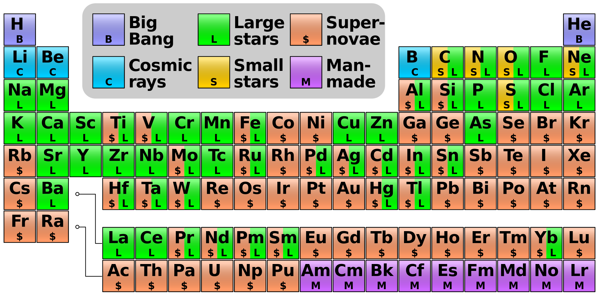
Periodic table showing the origin of each chemical element. Those produced by the r-process are shaded orange and attributed to supernovae in this image; though supernovae are one proposed source of r-process elements, an alternative source is the merger of two neutron stars. [Cmglee]

Astronomers, much to the chagrin of chemists, refer to elements heavier than hydrogen or helium as “metals.” In fact, the most abundant “metals” in the universe, like oxygen and carbon, are not metals at all by the chemical definition. Nonetheless, today’s bite focuses on actual heavy metals. While many elements are forged either in the end stages of a massive star’s life in a core-collapse supernova or in the death of a white dwarf as a thermonuclear supernova, some elements must be produced in even more exotic ways. These methods include the s-process and r-process, referring to slow and rapid neutron capture, respectively. The s-process occurs in stars — in particular, in asymptotic giant branch (AGB) stars, the very end stages of a low mass star’s life. The r-process, however, requires many more neutrons to be captured quickly. There are two possible channels for the r-process: binary neutron star mergers and exotic supernovae.

To date, astronomers have studied the presence of heavy elements primarily by looking at the spectra of stars and measuring chemical abundances. Recently, studies of r-process enhanced stars — stars with unusually high abundances of r-process-formed elements — have suggested that many of these stars were born in dwarf galaxies and later accreted onto the Milky Way. To test this scenario and better understand the physics behind r-process enhanced stars, the authors of today’s paper turned toward our neighbor, the massive dwarf spheroidal galaxy Fornax.

Odd Ones Out

In their study of the stellar populations of Fornax, the authors found three stars with significantly enhanced r-process elements as compared to the rest of the population. In particular, the abundance of the rare element europium (Eu) is roughly an order of magnitude higher than for other stars in Fornax. For this reason, the authors refer to them as Eu-stars. Figure 1 shows these Eu-stars compared with normal Fornax stars and other r-process enhanced stars. There is a general trend between metallicity ([Fe/H]) and the absolute Eu abundances, which holds true for both the r-process enhanced and comparison stars, but here enhancement refers to a star lying significantly above the average Eu abundance at a given [Fe/H].

Interestingly, when the authors compare the alpha abundances (essentially the elements created in massive stars) of the Eu-stars and normal stars, they find that the r-process stars are not alpha-enhanced (see Fig. 2 in the paper). This suggests that either the Eu found in the r-process enhanced stars was produced by a neutron star merger (due to the lack of helium in these systems) or that the supernova that produced the Eu created similar amounts of alpha elements to other supernovae.

Two-panel plot of abundances.

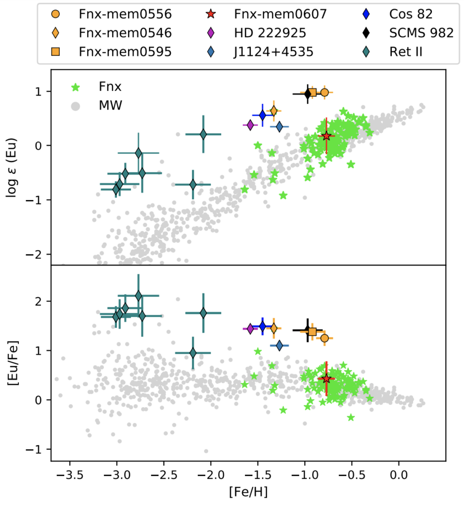
Figure 1: Three stars in Fornax have significant enhancement in Eu as compared to other Fornax stars. Top panel: Absolute Eu abundances as compared to the stellar metallicity. Bottom panel: Eu abundances (relative to the iron abundance) as compared to the stellar metallicity. The gray points are Milky Way stars and the green stars are Fornax stars. The bolded points are all r-process enhanced, with the three stars in Fornax shown in yellow. The other bolded points are r-process enhanced stars in other galaxies. A value in brackets indicates a logarithm with a value of 0 being the same as the Sun. [Reichert et al. 2021]

Confirming an r-Process Origin

Neutron capture elements like Eu can be created both with the r-process and s-process. To test the origin of Eu in the Eu-stars, the authors make use of the barium to europium ratio ([Ba/Eu]). When the r-process is dominant, this ratio is low. Conversely, a high [Ba/Eu] ratio indicates significant s-process contribution. As can be seen in Figure 2, the [Ba/Eu] ratio for the Eu-stars are all below –0.7 dex, indicating a pure r-process origin. In contrast, the comparison stars in Fornax lie at high values, indicating a combination of r-process and s-process neutron capture.

plot of the barium to europium ratio.

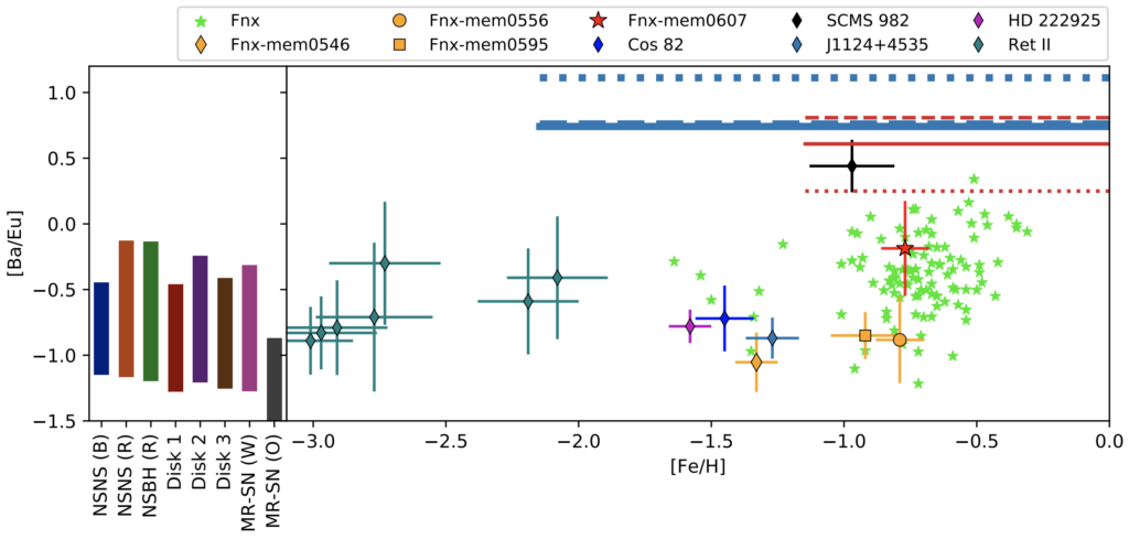
Figure 2: The Eu-stars in Fornax are consistent with an r-process origin rather than an s-process origin. Barium to europium ratio as compared to the stellar metallicity. The bars in the left panel represent various simulations of r-process events, whereas the lines in the right panel indicate predictions from s-process events. The shapes and colors of the points have the same meaning as in Figure 1. [Reichert et al. 2021]

With the knowledge that the Eu-stars were enriched by the r-process, the authors wanted to know what kind of event led to the r-process enhancement. To do this, they computed the Eu mass needed to explain the Eu-stars, finding a mass of ~10–5–10–4 solar mass. They also find that one r-process event is sufficient to explain the existence of three Eu-stars without a substantially larger population of r-process enhanced stars in Fornax. Figure 3 shows the expected Eu yields from neutron star mergers and supernovae. However, given the uncertainties involved in the theoretical modeling of these events, the authors cannot definitively state whether neutron star mergers or supernovae are responsible for the Eu-stars.

plot showing absolute Eu abundance of stars created from an r-process event

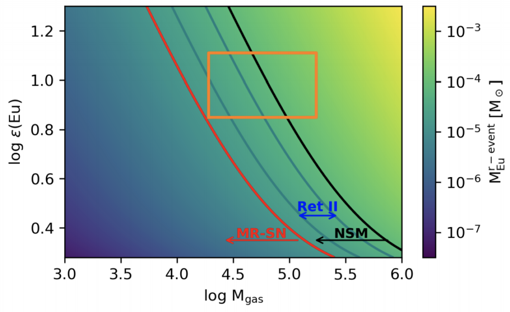
Figure 3: Either a neutron star merger or an exotic supernova can explain the Eu-stars in Fornax. Absolute Eu abundance of stars created from an r-process event as compared to the total gas mass affected by the r-process event. The shading represents the Eu mass created, with the black and red lines indicating theoretical predictions for neutron star mergers and supernovae respectively. The yellow box shows the approximate region corresponding to the Eu-stars in this study. [Reichert et al. 2021]

Today’s paper has taken a deep look at the dwarf galaxy Fornax, which may represent one of the environments where stars with large amounts of heavy elements are made. They find three so-called Eu-stars and confirm an r-process origin, but they are unable to pinpoint the physical event creating the excess neutron capture material. Absent more observations of neutron star mergers like GW170817, detailed studies of stars represent our best way of understanding neutron capture processes. While this paper represents a large step towards understanding the most extreme stars and heavy element creation, as with many things in astronomy, we must continue to find more objects to study!

Original astrobite edited by Ishan Mishra.

About the author, Jason Hinkle:

I am a graduate student at the University of Hawaii, Institute for Astronomy. My current research is on multi-wavelength photometric and spectroscopic follow-up of tidal disruption events. My research interests also include a number of topics related to AGN, including outflows, X-ray spectroscopy, and multi-wavelength variability. In addition to my love for astronomy, I enjoy hiking, sports, and musicals.

Illustration of a stellar binary in which a compact object surrounded by a disk is siphoning matter off of a large, reddish star.

Editor’s note: Astrobites is a graduate-student-run organization that digests astrophysical literature for undergraduate students. As part of the partnership between the AAS and astrobites, we occasionally repost astrobites content here at AAS Nova. We hope you enjoy this post from astrobites; the original can be viewed at astrobites.org.

Title: Classical Novae Masquerading as Dwarf Novae? Outburst Properties of Cataclysmic Variables with ASAS-SN
Authors: A. Kawash et al.
First Author’s Institution: Michigan State University
Status: Accepted to ApJ

Who Is Who

My favorite star is a cataclysmic variable star, or Gillian Anderson, depending on the context of the question. This type of variable star is my favorite, because it’s actually a binary star system, instead of just a single star. In this system, a white dwarf accretes matter from a donor star, usually (but not always) one on the main sequence. In most cases, an accretion disk will also form around the white dwarf. See the cover image above for an illustrated example. Sometimes explosions will occur within the binary, and they’re called “novae.” A “classical nova” (CN; CNe plural) happens on the surface of the white dwarf and is caused by thermonuclear runaway. A “dwarf nova” (DN; DNe plural) happens in the accretion disk and is thought to be caused by thermal instabilities. It’s important to remember that although they might sound similar, novae are very different from supernovae and should not be confused.

Using observations of galaxies like ours (Andromeda, for example) and theoretical models, we can predict how often we should expect to see a CN. Unexpectedly, the observed detection rate is significantly below the theoretical detection rate. The authors of today’s paper hypothesize that maybe this isn’t because we aren’t detecting them; instead, maybe we do see CNe but just misclassify them. DNe are one of the most common types of galactic transient and come from the same star type as CNe, so maybe we’re just confusing the two.

Stop and Stare at the Sea of Smiles Around You

Before immediately testing the sample of all known DNe, the authors wanted to create a baseline for what they expected to find. Two of the most important characteristics of a nova — dwarf or classical — are the time it takes to become fainter by two magnitudes from peak brightness (called “t2” in this paper) and the magnitude difference between peak and quiescent brightness (called the “outburst amplitude”). There are 9,333 (more now!) DNe in the VSX catalog, one of the largest variable star catalogs. The authors compared this to the ASAS-SN catalog of variable star light curves and selected the 2,688 that were observed during outburst. The ASAS-SN telescopes are only sensitive to luminosities brighter than 18 magnitudes, and so to get robust quiescent magnitudes, the authors further trimmed the sample to the 1,617 DNe that were also detected in the (more sensitive) Pan-STARRS catalog. To create a sample of 132 CNe, 40 were selected using the method above to be combined with a 92 CNe sample from Strope et al. (2010).

Let the Spectacle Astound You

Like any reasonable scientist, after the authors collected all their data, they plotted it! Visually, you can see a separation between the two samples (CNe in red & DNe in blue) in Figure 1. On average, CNe had an outburst amplitude of 11.43 ± 0.25 magnitudes, while DNe had an outburst amplitude of 5.13 ± 0.04 magnitudes. Furthermore, the authors found a 15% overlap in the outburst amplitude. The results for t2 were a little more complicated. The CNe had a t2 value of 18.7 ± 1.9 days, but the DNe sample needed to be split into a “fast” group (~12% of the sample) and a “slow” group (~88%). The average DNe t2 values were 2.4 ± 0.2 days and 10.5 ± 0.2 days, respectively. The authors were able to find fits to both samples in the form of log(t2) = B*(Amp – <Amp>) + a. The fit to the CNe sample was not very significant (~3σ) and had a negative slope (B = –0.083), while the fit to the DNe sample was very significant (~10σ) and had a positive slope (B = 0.061).

Basically the two samples are distinct, but there’s enough overlap that maybe we’re misclassifying CNe as DNe. Colloquially, they’re saying there’s a chance.

Plot describing properties of novae.

Figure 1: Comparison of the outburst amplitude to t2 (the time it takes to reduce by 2 magnitudes from peak brightness). CNe are shown in red, while DNe are shown in blue. [Kawash et al. 2021]

Hide Your Face So The World Will Never Find You

Once the authors knew what to look for, they critically analyzed the 2,688 ASAS-SN DNe sample. From analysis of the CNe luminosity function from Shafter 2017, the authors determined that a transient must have an absolute magnitude brighter than –4.2. Using apparent magnitudes from ASAS-SN, distance constraints, and dust extinction estimates, the authors were able to eliminate all but 201 novae in the sample from being (possible) CNe. They further reduced this sample to 94 after eliminating those that were quickly recurrent and those with outburst amplitudes less than an apparent magnitude of 5. These cuts were made since no classical nova is known to recur on timescales less than a decade and 5 was the lowest apparent magnitude limit on the CN outburst amplitude (from Figure 1). Finally, all but 27 of these 94 are spectroscopically confirmed DNe. To analyze the remaining 27, the authors used “quiescent multi-band photometry.” If a source is pretty blue, it’s likely to be close by and therefore likely to have a lower luminosity during outburst (hence, likely to be a DN), and if it’s red, it’s probably further away and is more likely to have a higher luminosity during outburst (hence, likely to be a CN). Basically, blue sources are DNe, and red sources are CNe. Using this method, the authors found that 19 novae are consistent with DNe, 0 are consistent with CNe, and 8 are ambiguous. So, at most 8 out of 2,688 — or 0.29% — of ASAS-SN classified DNe could be CNe.

To quote the authors, “the transient community appears to be doing an effective job classifying CV (cataclysmic variable star) outbursts.” Sadly this means that there is no masquerade and another explanation (maybe dust extinction?) is needed to explain the missing CNe.

Original astrobite edited by Gloria Fonseca Alvarez.
A French translation of this article is available on Astrobites, written by Celeste Hay.

About the author, Huei Sears:

Huei Sears is a third-year graduate student at Northwestern University studying astrophysics! Her research is focused on gamma-ray burst host galaxies. In addition to research, she cares a lot about science communication, and is always looking for ways to make science more accessible. In her free time, she enjoys walking along the lake, listening to Taylor Swift, & watching the X-Files.

Illustration of a bright ring of material surrounding a dense, textured, reddish bubble.

Editor’s note: Astrobites is a graduate-student-run organization that digests astrophysical literature for undergraduate students. As part of the partnership between the AAS and astrobites, we occasionally repost astrobites content here at AAS Nova. We hope you enjoy this post from astrobites; the original can be viewed at astrobites.org.

Title: Indication of a Pulsar Wind Nebula in the hard X-ray emission from SN 1987A
Authors: Emanuele Greco et al.
First Author’s Institution: University of Palermo, Italy
Status: Accepted to ApJL

In 1987 astronomers witnessed the closest supernova in almost 400 years, subsequently called SN 1987A. At only 51.4 kiloparsecs (or about 167,000 light-years), SN 1987A’s home is in the Large Magellanic Cloud, and it was visible in the Southern Hemisphere with the naked eye for a few months before it faded. But one question that remains unanswered is what kind of object was left behind. The original star that created SN 1987A was a blue supergiant, which would have left behind either a black hole or a neutron star. Yet even with decades of observations by many telescopes spanning the electromagnetic spectrum, its nature has yet to be confirmed.

Why are astronomers still trying to figure out what was left behind in SN 1987A? One reason is that it would let us learn more about neutron star and black hole formation and the mechanics of supernovae. Another reason is that if this leftover object happens to be a pulsar, a neutron star that emits radio (and potentially X-ray or gamma-ray) pulses, then we would be able to observe its very early, formational years, which we know very little about. Recent work (like that discussed in this astrobite) suggests that a neutron star is the likely remnant, but we can’t say for sure. The authors of today’s paper attempt to confirm once and for all that the leftover remnant of SN 1987A is a neutron star.

Look with Your X-ray Eyes

To determine the nature of the object at the center of SN 1987A, the authors use X-ray observations taken between 2012 and 2014 by the Chandra X-ray Observatory, which observes X-ray photons between 0.1 and 10 keV, and NuSTAR X-ray telescope, which observes X-ray photons between 3 and 79 keV (though the full range of each telescope is not necessarily used in the analysis). The images of SN 1987A from these telescopes are shown in Figure 1, with redder colors representing more photons detected.

Three panels show different X-ray views of SN 1987a and the background X-ray radiation.

Figure 1: X-ray images of SN 1987A where redder colors represent more X-rays. Left: Image from the Chandra X-ray Observatory from 0.1–8 keV. The cyan circle shows SN 1987A, and the red circle shows the noise level of the background X-rays. Since the background is almost completely black, there is very little noise. Center: A zoom-in of the left panel. The X-ray dim center of SN 1987A is shown by the black circle in the center. Right: The NuSTAR image from 3–30 keV. SN 1987A is circled again in cyan, and the slightly noisier background is circled in red. SN 1987A still clearly stands out above the background. [Greco et al. 2021]

The authors then analyzed the X-ray spectra, or number of photons observed at each energy, of SN 1987A between 0.5 and 20 keV, shown in Figure 2. By fitting different models to these spectra, they can determine what the source of the X-ray emission might be. The authors tested two primary models. The first one models the X-ray emission with two thermal components, each caused by high-energy Bremsstrahlung radiation. These components are essentially caused by two groups of highly energetic particles (usually electrons) that can each be described by a characteristic temperature and are of high enough energy to emit X-rays.

The second model is the same as the first, but it also includes a model for a highly absorbed pulsar wind nebula (PWN). PWNs are astronomical winds of charged particles accelerating close to the speed of light around a pulsar, and they are known to give off high energy X-rays. Being highly absorbed means that very few of the X-rays emitted by a PWN would escape the gas and dust that make up the supernova remnant of SN 1987A; most are reabsorbed instead. The authors compute the residuals by subtracting these best-fit models from the X-ray spectra, shown in the bottom panels of Figure 2. The closer these residuals are to zero, the better the model. If this second model fits much better than the first, then the authors can say that there is very likely a PWN, and hence a neutron star, at the center of SN 1987A.

Two plots showing X-ray spectra and the two different models.

Figure 2: Combined X-ray spectra showing the number of X-ray photons observed in each energy bin of all Chandra and NuSTAR observations over the span of three years with different colors for each observation. Spectra from Chandra span 0.5–8 keV, and spectra from NuSTAR span 3–20 keV. The bottom panels show the residuals, or the spectra after the best-fit models have been subtracted off. Left: Spectra with a best-fit model containing just two thermal components. One can see that there is an excess of photons at energies higher than 10 keV in the bottom panel, as shown by the points all above the bright green zero line. Right: Same as the left, but the best-fit model has an absorbed pulsar wind nebula component in addition to the two thermal components. The excess X-rays at energies > 10 keV appear to be accounted for here. [Greco et al. 2021]

So What’s at the Center?

Unfortunately, the authors were unable to conclusively answer that question. They found that the model that includes a PWN is statistically slightly better than the one without (shown by the better residuals in Figure 2 at energies > 10 keV), but not so much that they can say anything definitively. They were able to come up with a way that the higher energy X-rays might be produced without a PWN, but it involves an extremely energetic shockwave expanding steadily outwards at the fastest speeds allowed with no slowing down. While this is possible, it is an unlikely physical scenario compared to just having a neutron star at the center of SN 1987A.

Despite the uncertainty still surrounding the central object of SN 1987A, all is not lost! The authors also did some simulations showing that, if there really is a PWN at the center of SN 1987A, then by the 2030s, fewer of the lower energy X-ray photons will be absorbed, allowing these photons to be more easily detectable with Chandra or potential future X-ray observatories. So while the nature of what SN 1987A left behind remains a mystery for now, we are getting increasingly closer to solving it.

Original astrobite edited by Anthony Maue.

About the author, Brent Shapiro-Albert:

I’m a fourth year graduate student at West Virginia University studying various aspects of pulsars. I’m a member of the NANOGrav collaboration which uses pulsar timing arrays to detect gravitational waves. In particular I study how the interstellar medium affects the pulsar emission. Other than research I enjoy reading, hiking, and video games.

Lineup of five planets, including Earth, showing relative sizes of some known habitable-zone planets.

Editor’s note: Astrobites is a graduate-student-run organization that digests astrophysical literature for undergraduate students. As part of the partnership between the AAS and astrobites, we occasionally repost astrobites content here at AAS Nova. We hope you enjoy this post from astrobites; the original can be viewed at astrobites.org.

Title: Bridging the Planet Radius Valley: Stellar Clustering as a Key Driver for Turning Sub-Neptunes into Super-Earths
Authors: J. M. Diederik Kruijssen, Steven N. Longmore, & Mélanie Chevance
First Author’s Institution: Center of Astronomy, Heidelberg University, Germany
Status: Published in ApJL

Neptunes and Jupiters and Earths, Oh My!

Extrasolar planets, or exoplanets, have been theorized for centuries, and studied firsthand since the 1990s. Much of the common classification of exoplanets is based on analogs in our own solar system: hot Jupiters, super-Earths, and super-Jupiters, just to name a few. The authors of today’s paper focus on two types of exoplanets: super-Earths (planets with more mass than Earth but less mass than Neptune) and sub-Neptunes (planets of 1.7–3.9 times the size of the Earth, but with a composition similar to Neptune’s).

plot of number of planets per star vs. planet size shows a distinct valley between 1.5 and 2 earth radii.

Figure 1: A histogram of planets with given radii from a sample of 900 Kepler systems. The decreased occurrence rate between 1.5 and 2.0 Earth radii is apparent. [Fulton et al. 2017]

Between these two classes of exoplanets, there is a radius “valley” in the range 1.5–2.0 Earth radii where the occurrence rate of known exoplanets is much lower. Since we can observe exoplanets above and below this radius, it’s unlikely that the valley is a result of observational limitations, so a physical mechanism is probably to blame. There are three main theories about the cause of the radius valley: photoevaporation, core-powered mass loss, and the planet forming with no gaseous outer layer to begin with (otherwise known as rocky planet formation). In a photoevaporation scenario, X-ray and/or extreme ultraviolet radiation from the host star cause the gaseous layers of a larger planet to evaporate, leaving behind only a rocky core. Photoevaporation can also destroy gasses in the protoplanetary disk, which may also impact planetary formation. In core-powered mass loss, the energy radiated during the cooling of the rocky core erodes the gas envelopes of sub-Neptune-sized planets, again leaving behind the core. Rocky planet formation is exactly what it says on the label: a rocky planet is directly produced with no gaseous layers and no evolution required. All of these theories consider only properties and dynamics within the star–planet system. Today’s authors investigate the potential effects of stellar clustering on planet formation as a cause of the radius valley.

Compiling the Sample

The authors analyze a sample of exoplanets from the NASA Exoplanet Archive with radii of 1–4 Earth radii and orbital periods of 1–100 days. These radii and periods are chosen so that they only analyze planets that have had these values directly measured rather than derived from mass–radius relationships. The density of stars around the planet’s host star is part of the archival data, and the sample is split into “field” and “overdensity” subgroups that consist of low stellar density and high stellar density host star regions, respectively. In this case, what constitutes low and high densities is determined by the probability of there being many stars within 40 pc of the system: field stars have an 84% probability that there aren’t many neighboring stars, and overdensity stars have an 84% probability that there are. Additionally, only systems with ages of 1–4.5 billion years are considered, since younger systems may not be stabilized and the overdense group is too small in older systems. Finally, they constrain the host star mass to 0.7–2.0 solar masses to limit the chance of observing effects that are actually caused by mass differences rather than stellar clustering. With these cuts, the authors are left with 8 field planets and 86 overdensity planets, for a total of 94.

Results

Three panel plot showing properties of the planets in the authors’ sample. See caption for details.

Figure 2: Left: The orbital periods and radii of the planets. The radius valley is marked with the black line, and its uncertainty is given by the grey stripe. Center: The planetary radii versus the density of their stellar fields, with the grey line representing a constant radius. Right: A histogram of how many planets have each radius. Note that the radius is plotted on a logarithmic scale in all three panels. [Kruijssen et al. 2020]

Simply plotting the densities and radii suggests that the authors’ idea holds up (Figure 2). In the middle panel, the gray line represents a constant radius within the radius valley. The fact that there are fewer planets around this line shows the radius valley exists, but how does that prove their idea? The field stars all lie above the radius valley, while a little more than half of the overdensity stars lie below the radius valley. If residing in a dense field can cause dynamic and radiative effects that decrease the planet’s radius, having more small planets in overdense regions is expected.

But what if it’s really the effect of some other properties of the systems? Comparing the planets’ host star masses, metallicities, and ages shows no clear differences that might suggest the trend is caused by one of those characteristics. This data is compiled in Table 1. But what about the distance from Earth to the system? The further from Earth a system is, the less likely we are to be able to observe smaller planets. Could that be a factor skewing the numbers, since that could mean we just aren’t seeing the smaller planets? On average, the field systems are closer to Earth, but all of their planetary radii lie above the valley. The authors therefore conclude that the distance is probably not a contributing factor either.

Table of the characteristics of the authors' planet subsample. See caption for details.

Table 1: Characteristics of the sample planets. The authors split the sample into three groups: field planets, overdensity planets with radii above the radius valley, and overdensity planets with radii below the radius valley. The median stellar masses, metallicities, ages, and distances from Earth for each group are given with their uncertainties. The authors conclude that these values are all close enough to suggest that they are not the cause of the radius valley. [Kruijssen et al. 2020]

But what about those other mechanisms we discussed earlier? The authors consider photoevaporation within the system, mass loss, and rocky formation alongside the potential effects of densely clustered stars near the system. They conclude that stellar clustering alone can’t be responsible for the trends seen in planetary radius, but alongside one of the other three theories, clustering is certainly a potential contributor to the radius valley. The clustering would, however, affect each of the three scenarios differently. For the rocky core mass loss scenario, it is unlikely that clustering has any direct effect, since that mechanism is purely internal to the planet. The likelihood of rocky planet formation, on the other hand, can be increased by clustering effects, since neighboring stars could cause photoevaporation within the protoplanetary disk. This would decrease the amount of gas in the disk, increase the dust-to-gas ratio — the ratio of solid particles to gaseous particles in the disk — and thus increase the likelihood of rocky formation. Additionally, clustering could cause more stellar encounters with the system, which in turn could change the orbits of the planets and the effects of photoevaporation inside the system.

In this paper, the authors conclude that, in addition to previous theories, the dynamic and photoevaporative effects of stars near planetary systems can contribute to the radius valley between super-Earth and sub-Neptune exoplanets. Although this doesn’t provide definite answers to why this valley exists, it provides another piece to the puzzle. Solving the mystery of this radius valley can give us more insight into planetary formation mechanisms in extrasolar systems.

Original astrobite edited by Mike Foley.

About the author, Ali Crisp:

I’m a third year grad student at Louisiana State University. I study hot Jupiter exoplanets in the Galactic Bulge. I am originally from Tennessee and attended undergrad at Christian Brothers University, where I studied physics and history. In my “free time,” I enjoy cooking, hiking, and photography.

Image of a galaxy with a long, streaming tail stretched out behind it.

Editor’s note: Astrobites is a graduate-student-run organization that digests astrophysical literature for undergraduate students. As part of the partnership between the AAS and astrobites, we occasionally repost astrobites content here at AAS Nova. We hope you enjoy this post from astrobites; the original can be viewed at astrobites.org.

Title: Spectacular HST observations of the Coma galaxy D100 and star formation in its ram pressure stripped tail
Authors: William J. Cramer et al.
First Author’s Institution: Yale University
Status: Published in ApJ

Galaxy clusters are the largest gravitationally bound structures in the universe, exceeded in size by only the vast cosmic web in which they are embedded. Clusters contain anything from hundreds to thousands of galaxies, which they accrete due to gravity, and they can reach several megaparsecs in size. However, galaxy clusters are not gentle giants. These huge objects contain extremely hot X-ray-emitting plasma, and they can produce gravitational tidal forces strong enough to tear galaxies apart.

Because of these cluster properties, galaxies in clusters and galaxies elsewhere in the universe (called field galaxies) can differ dramatically. Galaxies that have entered a cluster environment are more often elliptical, have low star formation rates, and contain very little gas (from which new stars are formed). This so-called morphology–density relation has been well-established for decades — and although a whole host of theories exist, the specific causes of it are still unclear.

Enter Cramer et al., the authors of today’s paper.

This work presents observations of ram-pressure stripping, a mechanism that can explain the evolution of galaxies from gas-rich to gas-poor when entering a cluster. A galaxy moving through a medium (in this case, the hot intracluster plasma) can have loosely bound gas removed by drag forces from that medium. Imagine what it would look like if you poured a bag of flour over your head, and then stuck your head out of the window of a fast-moving car (not that I’d recommend this).

Along Came a Jellyfish

The authors’ evidence for ram-pressure stripping comes in the form of a jellyfish galaxy. In this case, they examine D100, a barred spiral galaxy close to the centre of the Coma cluster. Jellyfish galaxies represent an extreme example of ram-pressure stripping, where the stripped gas streams out in a long tail behind the galaxy, giving them their distinctive look. Think back to the flour-head-car-window example — you would probably expect to see something similar.

Left: composite photograph of a galaxy with a long, trailing red tail. Right: photograph of a jellyfish with a bright head and long, trailing tentacles

Figure 1: Left: Composite image of D100 galaxy, showing the stripped gas trailing the galaxy disc, which is moving from left to right in this image. Right: A jellyfish, for comparison. [Left: Cramer et al. 2019; right: Alexander Semenov]

Using new Hubble Space Telescope (HST) observations, this work examines both the galaxy and the long tail trailing behind, which contains far fewer stars than the main galactic disc, and so is much fainter. The photo of D100 in Figure 1 is a composite image, combining the HST observations of starlight with observations of the emission line from the Subaru telescope that show the presence of excited hydrogen gas. This Hα emission is shown in bright red, and demonstrates the dramatic effect that the Coma cluster is having on this galaxy.

Hα emission from galaxies is often an indicator of ongoing star formation (although it can have other sources). However, it is the combination of Hα measurements and the powerful HST observations that make this work possible. Thanks to the exceptional resolution of Hubble, and the authors’ multiple observation bands — F814W (red/near-IR wavelengths), F475W (blue) and F275W (near-UV) — Cramer and collaborators are able to study not only how much star formation is taking place, but also where in the tail this is happening.

A Tail of Three Bands

The authors’ colour analysis shows that star formation stopped long ago in the galaxy outskirts, but has stopped more recently closer to the centre, and it is ongoing in the core. This indicates that the star-forming gas was removed from the galaxy outskirts first, causing outside-in quenching.

Photograph of a nearly face-on spiral galaxy with a stream of dark dust extending from its center.

Figure 2: HST image of D100. Arrow is pointing to a star-forming clump, embedded in a dark region of dust that is also being stripped. [Adapted from Cramer et al. 2019]

A zoom-in on the HST image (Figure 2) also reveals a small, bright patch, located in a cloud of dust. The colour of this patch, which is bright in the blue and UV bands and fainter in red, indicates that it is a clump of ongoing star formation. In fact, the HST observations find 37 bright patches (shown in Figure 3), and analysis of their colours shows 10 of them to be clumps of star formation, all of which are found in the tail of gas. The 27 other sources are mostly background sources, such as distant galaxies.

map showing D100 and the locations of 37 other bright sources around it, as well as outlines of the streamer emitted from the galaxy's center.

Figure 3: Map of 37 bright sources around D100. Those labelled in blue/underlined are star-forming clumps [Cramer et al. 2019]

The main conclusion of the paper is that the stripped gas can form stars outside of the galactic disc, but that it doesn’t form them uniformly throughout the tail. Instead, stars form in these clumps, which are up to 100 parsecs in size. The brightness of these regions is, however, insufficient to produce all of the Hα emission that is observed. This indicates that another mechanism (such as gas shocks) must be responsible for some of this emission, but the precise nature of this mechanism remains, for now, a mystery.

Although this paper is a convincing endorsement of ram-pressure stripping, it is important to note that ram-pressure alone is not enough to explain all of the differences between cluster and field galaxies. For example, it provides no explanation of why disc galaxies are rarer in clusters. A full description of the relationship between galaxies and their environments is likely to be a complex combination of different effects, in which ram-pressure stripping will play a small, but important, role.

Original astrobite edited by Alex Gough and Kate Storey-Fisher.

About the author, Roan Haggar:

I’m a PhD student at the University of Nottingham, working with hydrodynamical simulations of galaxy clusters to study the evolution of infalling galaxies. I also co-manage a portable planetarium that we take round to schools in the local area. My more terrestrial hobbies include rock climbing and going to music venues that I’ve not been to before.

image showing a map of the Milky Way from Gaia data, with an overlaid sinusoidal stream of stars.

Editor’s note: Astrobites is a graduate-student-run organization that digests astrophysical literature for undergraduate students. As part of the partnership between the AAS and astrobites, we occasionally repost astrobites content here at AAS Nova. We hope you enjoy this post from astrobites; the original can be viewed at astrobites.org.

Title: The Spur and the Gap in GD-1: Dynamical Evidence for a Dark Substructure in the Milky Way Halo
Authors: Ana Bonaca, David W. Hogg, Adrian M. Price-Whelan, and Charlie Conroy
First Author’s Institution: Center for Astrophysics | Harvard & Smithsonian
Status: Published in ApJ

Suppose I told you that a fire-breathing dragon lives in my garage, but I cannot show you the dragon because it is floating, invisible, and spits heatless fire. You would not believe that I had any dragons at all. Carl Sagan, the creator of this analogy, argues that my claim of the dragon only makes sense if there is some experiment that could disprove it. In other words, scientific claims have to be testable. Now take a look at the theory of dark matter: astronomers say that the Milky Way is full of invisible blobs of dark matter called subhalos, which only interact with normal matter through gravity. However, this claim sounds a lot like the invisible dragon in my garage unless there is some way to observe the effects of those subhalos.

You would expect the dragon in my garage to leave evidence of footprints or breathing fire. One way to detect the invisible subhalos, used by the astronomers of today’s paper, is by observing stellar streams. Stellar streams are groups of stars that have been stretched out on their orbit in the outer region of the Milky Way. If a subhalo flies into a stellar stream, the gravitational interactions can rip a hole in the stellar stream. The disrupted stars then fly away from the hole, and observers on Earth would see them piled up into a spur (see Figure 1). This method was previously used on the Pal 5 stellar stream, but the evidence was not conclusive to prove that the stream was disturbed by a subhalo. The authors today have the advantage of a clear view of the GD-1 stream from the Gaia space telescope, as described in this Astrobite. In the Gaia data, a spur and a gap are clearly visible in the stream, which points to possible interactions with a dark matter subhalo.

two plots showing the positions of the stars in the GD-1 stellar stream and a model of a subhalo-perturbed stream. two gaps are visible in the stream in both plots, as well as a parallel spur of stars above the main stream.

Figure 1: Top: Positions of stars in the GD-1 stream, observed by the Gaia space telescope. The spur and gaps are labeled with arrows. Both axes indicate the projected sky position of stars along and perpendicular to the stream orbit. Bottom: Positions of stars in a model where GD-1 was perturbed by a dark matter subhalo 495 million years ago (subhalo parameters shown in the legend). These two panels are in excellent agreement. [Bonaca et al. 2019]

The high spatial resolution and precision of the data allows the authors to create a model of the orbital history of GD-1. The motion of the stars is determined by the gravitational field throughout the orbit, which, in this case, is the well-studied Milky Way gravitational field plus any potential perturbers, such as dark matter subhalos, molecular clouds, and globular clusters. Thus, the map of the stellar stream encodes useful information about past interactions. The authors ran a suite of simulations, changing the mass and velocity of the perturber, how far away it was at closest approach, and the time of the encounter. The code used to calculate the orbit of stars is publicly available for interested readers.

stellar stream

Figure 2: Artist’s impression of a stellar stream arcing high in the Milky Way’s halo. [NASA]

The best-fit parameters used to construct the final model are shown in the bottom panel of Figure 1. In this scenario, a dark matter subhalo with 5 million solar masses came within 15 pc of the stellar stream, at a velocity of 250 km/s, and this event happened 495 million years ago. This dense, massive, high-velocity flyby gave the stars a velocity kick, which made a gap. The perturber also kicked the stars perpendicular to the stream motion and set some stars on a loop around the original unperturbed orbit, producing the spur when viewed in projection. Is this excellent agreement with observational data a sign of the elusive dark matter dragon?

The authors ruled out the possibility that the perturber is a known object. They traced the known orbits back in time for Milky Way globular clusters, satellite dwarf galaxies, and the Milky Way disk. No known object came close enough to GD-1 to produce the observed spur and gap. Thus, the authors conclude that a dark matter subhalo is the most probable perturber that caused the spur and the gap.

While this evidence is compelling, the authors want other independent ways of confirming the nature of the perturber. They highlight that this hypothesis is testable by measuring the radial velocities of the stars. The authors matched their models to observations using spatial position alone, which means the accepted models can have the stars at the same location but moving with different radial velocities. Future data from the Hubble Space Telescope can observe the radial velocity of stars in this stream, and that will provide a further test for the different perturber models.

This paper used simulations to show that the observed spur and gap in GD-1 are most likely caused by dark matter subhalos. The authors demonstrated an exciting avenue to find the invisible subhalos, and future research may discover more properties of these subhalos and compare them to the predictions of dark matter theory. Perhaps the dark matter dragon isn’t so elusive after all.

Original astrobite edited by Catherine Manea and Keir Birchall.

About the author, Zili Shen:

Hi! I am a PhD student in Astronomy at Yale University. My research focuses on ultra-diffuse galaxies and their globular cluster populations. Since I came to Yale, I have worked on two “dark-matter-free” galaxies NGC1052–DF2 and DF4. I have been coping with the pandemic and working from home by making sourdough bread and baking various cookies and cakes, reading books ranging from philosophy to virology, going on daily hikes or runs, and watching too many TV shows.

Illustration of the TESS satellite in front of the distant Sun.

Editor’s note: Astrobites is a graduate-student-run organization that digests astrophysical literature for undergraduate students. As part of the partnership between the AAS and astrobites, we occasionally repost astrobites content here at AAS Nova. We hope you enjoy this post from astrobites; the original can be viewed at astrobites.org.

Title: Exploring Trans-Neptunian Space with TESS: A Targeted Shift-Stacking Search for Planet Nine and Distant TNOs in the Galactic Plane
Authors: M. Rice, G. Laughlin
First Author’s Institution: Yale University
Status: Published in PSJ

The Transiting Exoplanet Survey Satellite (TESS), which just recently finished its primary mission to search for planets around nearby, bright stars, has also provided a treasure trove of other information for astronomers. As it stares at the sky, waiting to catch the brief flicker of a distant planet passing in front of its host star, TESS’s steady, unwavering gaze catches everything from stellar pulsations, to gamma-ray bursts, to distant solar system objects tumbling through the dark.

Illustration of a dark body in the distant outer reaches of the solar system.

Artist’s rendering of the hypothetical Planet Nine in the outskirts of our solar system. [Caltech/R. Hurt, IPAC]

It has been hypothesized that among these distant solar system bodies lies a ninth planet orbiting our Sun. To date, searches for this hypothetical world have turned up little of interest, but with an expected size not much larger than the Earth, and an orbit that is thought to be ~10x as distant as Neptune, “Planet Nine” would appear incredibly faint, due to the small amount of sunlight that reaches it. Furthermore, if it happens to lie near the star-studded galactic plane on the sky, it would be incredibly difficult to pick out in images.

An image of Planet Nine could be in some of the many exposures that TESS has already taken, although likely not in plain sight. Given that TESS takes 30-minute exposures of each patch of sky, the signal from our distant solar system companion would probably be extremely weak and hard to detect. One way around this issue is to “stack” multiple exposures on top of each other. This acts to boost the signal from any faint sources in an image above any background noise from the camera. Unfortunately, even the most distant solar system bodies move across the TESS field of view between exposures. Because the object is in a different place in each image, you lose any benefit from simply stacking the images on top of each other in place.

To solve this problem, the authors of today’s paper make use of a clever technique called “shift stacking”. Although an object will appear at a different location on each exposure, one can shift the sequence of exposures in such a way that the same pixels on each image correspond to the location of the object. By doing so, the images can then be stacked and added together and an object too faint to be visible in a single image now pops out.

diagram showing the successive steps involved in shift-stacking images.

Figure 1: Top: An illustration of the process by which a series of images, taken at different times, are combined to convert a faint, moving source into a much brighter, single point. Bottom: When searching for an undetected source, the path on the image is unknown. In this case, the algorithm must try out different guesses for the correct trajectory. The “correct” path is the one that produces the strongest signal on the final image. [Rice & Laughlin 2020]

A diagram detailing this technique is shown in Figure 1. The shift-stacking process described above is shown in the top panel. The tricky part, however, is when you don’t know what the path of the object you’re searching for actually follows. In this case, one can use a computer algorithm to try out many different possible paths for the object (shown in the lower panel). The path that produces the strongest signal on the stacked image is likely the correct one.

Trying to guess the correct path for an undetected object can be slow ordeal. One simplification, however, makes this task much easier to conquer. Most outer solar system objects move incredibly slowly because they are so far from the Sun. They move so slowly, in fact, that their motion on the sky is almost entirely dominated by the Earth’s motion. This fact really helps to narrow down the range of possible guesses for the path of any undetected body. Because the Earth’s motion dominates, a body’s path across the images depends only on its distance from the Sun, and not on the specific shape of its orbit.

plots showing multiple results of shift-stacking analysis

Figure 2: An application of the shift-stacking technique to three previously known outer solar system bodies: Sedna (top), 2015 BP519 (middle) and TG 422 (bottom). In the leftmost column, the known orbital parameters are used to calculate the trajectory of the object on the image. Next, the trajectory of the object is guessed using both a polynomial (middle) and PCA (right) technique to model the baseline flux. In all cases, the objects are recovered. [Rice & Laughlin 2020]

To verify the effectiveness of this shift-stacking technique, the authors first attempt to recover an image of three known outer solar system objects: Sedna, 2015 BP519, and 2007 TG 422. The resulting shift-stacked images of these bodies are shown in the left column of Figure 2. In these images, the object shows up as a bright point. Some of the shift-stacked images also contain prominent streaks. It turns out that these are caused by much closer and brighter asteroids that happened to pass through the field of view of the telescope.

Next, the authors attempt to recover these three outer solar system bodies without telling the algorithm ahead of time about the trajectories of these bodies. Instead, the algorithm tries to guess the path by maximizing the brightness of the point source in the shift-stacked images. This is shown in the middle and right hand columns of Figure 2. Here, “polynomial” and “PCA” refer to the technique used to subtract the baseline flux from the images. Although the polynomial technique is less computationally expensive, it sometimes results in the object itself being removed from the images.

Lastly, the authors apply their blind search algorithm to TESS sectors 18 and 19. Although this is only a small piece of the observing footprint of the telescope, these two sectors partially overlap with the galactic plane, which is where the shift-stacking technique is particularly useful. In total, the authors provide a list of 17 new outer solar system body candidates, which will need to be followed up with ground-based observations to confirm. From the TESS images, the distance, brightness, and size of the objects are estimated. Unfortunately, none appear anywhere near as large as what is expected for the hypothetical planet nine. It is, however, exciting that this technique finds so many new candidate objects from such a small search area. Presently, there are only about 100 known distant outer solar system bodies! Although this technique is quite computationally expensive to run, a more clever implementation that involves convolutional neural networks could allow this to be run on the entire sky.

Original astrobite edited by Bryanne McDonough.

About the author, Spencer Wallace:

I’m a member of the UW Astronomy N-body shop working with Thomas Quinn to study simulations of planet formation. In particular, I’m interested in how this process plays out around M stars, which put out huge amounts of radiation during the pre main-sequence phase and are known to host extremely short period planets. When I’m not thinking about planet formation, I’m an avid hiker/backpacker and play bass for the band Night Lunch.

VLA-COSMOS

Editor’s note: Astrobites is a graduate-student-run organization that digests astrophysical literature for undergraduate students. As part of the partnership between the AAS and astrobites, we occasionally repost astrobites content here at AAS Nova. We hope you enjoy this post from astrobites; the original can be viewed at astrobites.org.

Title: Illuminating the dark side of cosmic star formation two billion years after the Big Bang
Authors: M. Talia et al.
First Author’s Institution: University of Bologna & INAF, Italy
Status: Accepted to ApJ

The modern terminology of galaxies is extraordinarily anthropomorphic; blue, star-forming galaxies are “alive”, and red galaxies that have ceased star formation are “dead”. So then how do galaxies “live”? In other words, why do some galaxies form lots of stars while others do not? Are the dead galaxies older, or do they simply mature faster? What role do external forces such as galaxy mergers play in the lives of galaxies? How can their internal structures (bars, arms, and bulges) or internal forces (supernovae and active supermassive black holes) work to enhance or inhibit star formation? These details have been the focus of the past two decades of galaxy studies, trying to answer the question: How and when did galaxies assemble their mass of stars?

The highest-level diagnostic we can construct to help us understand the big picture of star formation in galaxies is the cosmic star formation rate density (SFRD) diagram. It maps the average rate at which stars are formed in the universe at a given time, per unit volume. The physics, then, is a matter of both supply and efficiency: how much gas is available to be formed into stars (supply), and how well did galaxies turn that gas into stars (efficiency)? Constructing the SFRD diagram can then help us to understand the interplay between gas and the processes that can act to enhance or inhibit star formation.

star formation rate density diagram

Figure 1: The star formation rate density diagram, including many literature measurements focusing on the early universe (z > 3). The results from this paper indicate that a missing population of galaxies might account for a large portion of the SFRD at z > 4. [Talia et al. 2021]

Although one can measure the rate of star formation in a given galaxy, and then extend that study to perhaps a hundred or even a million galaxies, one will never be able to count the number of stars forming in every galaxy at every point in the history of the universe. Such a census will be technologically impossible far into the future since our own Milky Way galaxy obscures the light from more distant galaxies one would need to measure. Despite these challenges, astronomers have found clever means of estimating the SFRD for ~75% of the history of our universe by carefully constructing unbiased, representative samples of galaxies such that specific inferences of that sample also hold for the general, wider population of galaxies. As shown in Figure 1, the SFRD rises for the first 3 billion years before peaking at a redshift of z ~ 2, after which it declines for the remaining 10 billion years until today.

Observing star formation rates during the first 2 billion years of the universe (z > 3) is incredibly difficult. Not only were the first galaxies intrinsically smaller and fainter than galaxies we see today, but starting at z ~ 6, the universe is pervaded by a dense fog of neutral hydrogen (from which galaxies formed!) that obscures their light. Given these difficulties, these incredibly early galaxies are only now being observed in large numbers.

The authors of today’s paper point out that the existing samples of z > 3 galaxies are not at all representative. For the most part, and almost exclusively at z > 6, these galaxies are discovered via their bright ultraviolet (UV) emission, which has been redshifted so that it is observed in the optical and infrared. Not only must these galaxies be incredibly bright to be found at such large distances, but their intensive UV emission translates directly to an enormous star formation rate. That is, the feature that makes them easy to find also makes their star formation rates high. This is a huge bias in our samples! To overcome this bias, the authors turn to radio wavelengths. They used a large radio survey VLA-COSMOS to find 197 radio sources that have no counterpart in near-infrared wavelengths. These, they argue, are heavily dust-obscured galaxies without any UV emission — the missing link.

Median galaxy template

Figure 2: Median galaxy template (top) fitted to stacked observations in many broadband filters (bottom). The derived average physical parameters, as well as the redshift distribution, are also shown. [Talia et al. 2021]

The authors’ first test was to stack the broadband brightness measurements of each galaxy together so that they can predict what the average total spectrum would look like for these galaxies, and hence their average properties. The lack of blue light on the left-hand side of the spectrum indicates that there is no luminous UV component as seen in the UV-bright galaxies of previous samples. Moreso, the authors estimate an incredibly high dust extinction of a whopping 4.2 magnitudes (nearly a factor of 50)! These galaxies are super dusty indeed.

Using a similar approach to the stacked analysis, the authors then estimate the redshift and star formation rate for each of the 98 galaxies for which they could reliably measure an infrared brightness. Due to their unique radio selection approach, the authors are able to compile a large sample of very high redshift galaxies at z > 4.5. They estimate the redshifts and star formation rates for the remaining 99 sources as well, but with much greater uncertainty.

Lastly, the authors compute the SFRD using their sample, taking care to correct for any dusty galaxies they may have missed. This is a challenging correction to make, so the authors do so by adopting an agnostic approach, seeing how their SFRD looks depending on how complete their sample might be.

As shown by the red bars in Figure 1, it is precisely this population of highly dust-obscured galaxies at z > 3, invisible to optical and infrared surveys, that may indeed constitute a significant portion of the star formation rate density in the early universe compared to other less-dusty samples!

These findings highlight the surprising extent of our missing knowledge of the first galaxies, and they encourage investment in future radio surveys with ALMA and follow-up with JWST.

Original astrobite edited by William Saunders with Lukas Zalesky.

About the author, John Weaver:

I am a second year PhD student at the Cosmic Dawn Center at the University of Copenhagen, where I study the formation and evolution of galaxies across cosmic time with incredibly deep observations in the optical and infrared. I got my start at a little planetarium, and I’ve been doing lots of public outreach and citizen science ever since.

RS Puppis

Editor’s note: Astrobites is a graduate-student-run organization that digests astrophysical literature for undergraduate students. As part of the partnership between the AAS and astrobites, we occasionally repost astrobites content here at AAS Nova. We hope you enjoy this post from astrobites; the original can be viewed at astrobites.org.

Title: Identifying Candidate Optical Variables Using Gaia Data Release 2
Authors: Shion Andrew, Samuel J. Swihart, and Jay Strader
First Author’s Institution: Harvey Mudd College
Status: Accepted to ApJ

The Wonders of Gaia

1.5 million kilometers from Earth, at the L2 Lagrange point, a space observatory not much larger than a car traverses space and gazes deeply into the Milky Way. Launched in 2013, Gaia tediously constructs a three-dimensional map of our galaxy. Its primary objective is to determine the brightness, temperature, composition, and motion of over a billion astronomical objects (mostly stars) … and I thought grad school was demanding!

Unlike many spacecraft, Gaia observes its targets frequently (~70 times). As a result, it offers the rare ability to expose the variability of the celestial bodies under its watchful eye. These observations provide us the opportunity to advance our understanding of stellar evolution and the dynamical nature of our galaxy’s constituents.

Isolating Variables

Well-studied variables, such as RR Lyrae, Cepheids, and long-period variables provide high-quality measurements; however, sources with short-term variability are harder to detect and limit the number of variables that are studied. In fact, from the Gaia Data Release Two (DR2), which is the instrument’s most recent data release that contains G-band photometry measurements for ~1.7 billion sources, information is only provided for 550,000 variable sources. To address this dearth of variability observations, the authors conduct a thorough review of variable stars that are confirmed in DR2. They contend that variable stars can be identified by targeting stars with relatively high photometric uncertainties. If so, this method may prove critical for building a robust sample of variable stars that can be used for future studies!

In Figure 1, the authors plot Gaia G-band magnitude vs. G-band magnitude uncertainty for 1,000 stars in a small region of the sky. The patch of the sky was centered on a well-studied RR Lyrae variable star, TY Hyi (G = 14.3). The “baseline curve”, where the bulk of the stars (the black dots) lie, is the expected distribution for non-variables. Away from this curve, the variable star (the red dot) has a much larger uncertainty than the stars with a similar brightness on the baseline curve.

Gaia DR2 stars

Figure 1. A G-band magnitude vs. G-band magnitude uncertainty plot of 1,000 DR2 stars showing the expected “baseline curve” along which most non-variable stars lie. The variable star (red dot) does not fall on the baseline curve, but instead has a noticeably larger G-band magnitude uncertainty than other stars of comparable magnitude. [Andrew et al. 2021]

In Figure 2, the authors expand their analysis and consider 70,680 variable stars with photometric periods < 10 days. They now also consider 2,000 random non-variable stars. In this plot, nearly all the variables lie above the baseline curve, with higher uncertainties compared to non-variable stars of similar magnitudes. Moreover, they find that stars with higher variability amplitudes feature higher uncertainties.

To note, the authors acknowledge that the G-band magnitude uncertainty varies with the number of observations (at fixed brightness, the uncertainty decreases as the number of observations increases), and they correct for this by using the weighted average of individual photometry measurements for each source.

variable stars in Gaia DR2

Figure 2: G-band magnitude vs. G-band magnitude uncertainty for 70,680 variable stars with periods less than 10 days, colored by their optical variability amplitude. The black points are a random sample of 2,000 stars, illustrating a baseline curve for non-variable stars. The dashed lines are the mean magnitude uncertainty of variables, in three bins from 0.0 to 1.2 mag in variability amplitude. [Andrew et al. 2021]

Exploring Other Catalogs

The authors then calculate a standard deviation, σ, from the baseline curve for sources using binned G-band magnitudes. They subsequently define a parameter, Gσ, which is the ratio of the G-band magnitude uncertainty in Gaia DR2 for a given source, to the σ for that bin. They use this parameter to define a threshold of Gσ = 3 for identifying variable stars.

But how effective is this method in finding short-period variables in Gaia’s DR2? To address this, the authors check the reliability of their newly defined threshold by scanning a series of short-period (<10 days) variable star catalogs with photometric G-band magnitudes between 14 and 19.5. They first inspect the Catalina Real-Time Transient Survey, which contains 70,680 variables. From their analysis, they find that 96% of the variables in this catalog have Gσ values > 3; the remaining 4% were masked because of potential contamination by a nearby neighboring star, which can generate false positives. Moreover, they inspect the Zwicky variable star catalog (see here for more on the Zwicky Transient Facility), which contains 556,521 variables. Similarly, they find a significant percentage (94%) are recovered when applying the Gσ > 3 threshold; the remaining 6% are also excluded because of neighboring stars.

Furthermore, this method also proves effective at identifying standard RR Lyrae and Cepheid variables (which can have periods up to 70 days). From Gaia DR2, they find that 100% of the Cepheids (8,465 sources) and 99.8% of RR Lyrae (107,418 sources) have Gσ > 3.

Confident in their method, they proceed to analyze the entirety of DR2, and they catalog 9.3 million candidate variable stars, a significant increase from the 550,000 sources reported in DR2 prior to this study.

Hidden No More

The authors of today’s paper provide an immensely powerful tool for identifying variable stars. They show that variable stars in Gaia’s latest data release, which contains over 1.7 billion sources, tend to have larger photometric uncertainties when compared to non-variable stars; more variable stars have larger photometric uncertainties, too. They quantify this relation with the parameter Gσ, which traces how far a star is from a baseline curve of non-variable stars. Using a threshold of Gσ = 3, they recover over 90% of short-period variables in other variable catalogs.

Variable stars have significantly contributed to some of the largest advances in modern astronomy: they have helped us define cosmological parameters, enhanced our understanding of the distance-scale of the universe, and provided us the information to calculate the ages of the oldest stars. Accurately identifying, and studying, these objects promise to unveil even more about our universe. Fascinating instruments like Gaia will serve as the bridges to these wonderful discoveries.

Original astrobite edited by Ellis Avallone.

About the author, James Negus:

James Negus is currently pursuing his Ph.D. in astrophysics at the University of Colorado Boulder. He earned his B.A. in physics, with a specialization in astrophysics, from the University of Chicago in 2013. At CU Boulder, he analyzes active galactic nuclei utilizing the Sloan Digital Sky Survey. In his spare time, he enjoys stargazing with his 8” Dobsonian Telescope in the Rockies and hosting outreach events at the Fiske Planetarium and the Sommers–Bausch Observatory in Boulder, CO. He has also authored two books with Enslow Publishing: Black Holes Explained (Mysteries of Space) and Supernovas Explained (Mysteries of Space).

cosmic clocks

Editor’s note: Astrobites is a graduate-student-run organization that digests astrophysical literature for undergraduate students. As part of the partnership between the AAS and astrobites, we occasionally repost astrobites content here at AAS Nova. We hope you enjoy this post from astrobites; the original can be viewed at astrobites.org.

Title: Eppur è piatto? The cosmic chronometer take on spatial curvature and cosmic concordance
Authors: Sunny Vagnozzi, Abraham Loeb, Michele Moresco
First Author’s Institution: Kavli Institute for Cosmology, University of Cambridge, United Kingdom
Status: Submitted to ApJ

Though astronomers have been studying the universe for hundreds of years, there are still a lot of things we do not know about it. We do not know whether it is finite or infinitely large, and we cannot determine its overall shape. Nevertheless, we know that we can describe the universe with a four-dimensional spacetime, the combination of our three-dimensional space and time. This spacetime is not rigid, but can be distorted and deformed by the content of the universe, like a bowling ball distorts a spandex sheet. The matter (and energy) also changes how the space part of spacetime is curved — and we can measure this curvature.

There are three possibilities for the curvature of the universe, illustrated in Figure 1: the universe can be closed, flat, or open. A closed universe would be shaped like a sphere (although with a three-dimensional surface), meaning that if you would walk along a straight line you would inevitably end up at the position on which you started. Also, if you and a friend start walking on parallel paths, your paths will cross at some point. An open universe is the “opposite” of this: the distance between you and your friend will increase with each step and you will never end up near each other. A flat universe is exactly in between these two cases: parallel paths stay at the same distance and never cross.

We characterize the curvature with parameter Ωk. Using the sign convention of the authors of today’s paper, a negative Ωk indicates a closed universe, a positive Ωk an open one. If the universe is flat, Ωk is exactly zero.

universe curvature

Figure 1: Different possibilities for curvature of the universe. The universe can be closed (top), open (middle), or flat (bottom). In the sign convention of today’s paper, a closed universe has Ωk < 0, an open universe has Ωk > 0. [NASA/WMAP]

In general, cosmologists predict that the universe is flat (Ωk = 0). This is not only suggested by a variety of measurements, but also a key prediction of the theory of cosmological inflation. Inflation describes a brief period during which the universe expanded exponentially (see this astrobite for more on inflation). The strong expansion of the universe decreased the curvature, in the same way that inflating a small balloon to the size of the Earth makes it appear flatter. Still, there is an ongoing debate on this issue. The Planck satellite tried to measure Ωk using the cosmic microwave background (CMB), remnant light from the early universe, which travelled through our potentially curved universe. The results suggest a Ωk between –0.095 and –0.007, so this measurement method points to a closed universe instead of flat. A reanalysis of Planck data confirmed this preference for a curved universe using the CMB.

However, the CMB on its own is not a sensitive probe for Ωk. It determines a combination of Ωk, the matter density in the universe Ωm, and the expansion rate H0, i.e., the Hubble constant. A strongly curved universe with a low value of H0 and a high value of Ωm can have the same CMB as a flat universe with a high H0 and a low Ωm. The fact that we can only measure H0, Ωm, and Ωk together and not individually from the CMB is called the geometrical degeneracy.

Cosmologists combine the Planck measurement with other probes, such as baryon acoustic oscillations (BAOs) or Type Ia supernovae. Combining the Planck data with BAO measurements from the Dark Energy Survey leads to Ωk = 0.0007 ± 0.0019, which is consistent with a flat universe.

The authors of today’s paper, though, believe that this combination of Planck and BAOs is not valid. They argue that the Ωk parameters inferred by each dataset on its own disagree so strongly, that the results of a combination of the data sets can be unreliable. If the results of two datasets are in strong tension, this could indicate that one or both include unknown systematic errors, or they need different models to be described. They should therefore not be combined. In case of the curvature of the universe, a different data set should be used to break the geometrical degeneracy. The choice of today’s authors: cosmic chronometers, the universe’s standard clocks.

Cosmic chronometers are objects whose time evolution we know (or can at least model very well), for example specific types of galaxies. We observe some of these objects at different redshifts, which indicate how far away they are. From the differences in their evolutional state, we then infer how much time has passed between the redshifts. This time difference tells us how fast the universe has expanded between the redshifts and gives the expansion rate H(z) at each redshift z. H(z) depends on the cosmological parameters, including Ωk, so from this we can infer the cosmic curvature.

Which objects can we use as chronometers? The best choice are passively evolving galaxies. These are galaxies that have exhausted their gas reservoir and form only a few new stars. Since blue stars die earlier than red stars, the galaxies become redder with time. From the galaxies’ spectral colours (more precisely, their spectral energy distributions) and sophisticated models of stellar evolution, we can infer how much time has passed since they exhausted their gas and stopped star formation. When we compare two galaxies that formed at the same time but are at different redshifts, the difference in their evolution tells us how much time has passed between the redshifts. We have found our cosmic clocks!

Today’s authors use 31 measurements of H(z) with cosmic chronometers between redshift z = 1.965 (approximately 10 billion years ago) and z = 0.07 (approximately 1 billion years ago). Figure 2 shows these measurements, along with the best fit for H(z) and the prediction from the Planck measurements. Planck underpredicts H(z), but the tension between the cosmic chronometers and Planck is much smaller than the disagreement with the BAO measurements. Therefore, the authors argue that combining the Planck and the cosmic chronometer data set is justified.

Hubble parameter

Figure 2: Cosmic expansion rate (also called Hubble parameter) at each redshift. The data points show the determination of the cosmic chronometer measurements used in the paper. The red line is the fit to the cosmic chronometer data combined with Planck; the blue line is the prediction of the Planck data alone. The Planck data underpredicts H(z) on its own. [Vagnozzi et al. 2020]

When the authors do so, they find the constraints on Ωm, Ωk and H0 shown in Figure 3. The combination of Planck and cosmic chronometers prefers a higher value of H0 than the Planck data on its own. However, this is not enough to alleviate the famous Hubble tension. Most important, though, the combined data finds Ωk = –0.0054 ± 0.0055. This value is consistent with a flat universe for which Ωk = 0, as predicted by cosmological inflation.

parameter constraints

Figure 3: Constraints on curvature of the universe (Ωk), the Hubble parameter (H0) and the matter density in the universe (Ωm) using only the Planck data (blue) or the combination of Planck with the cosmic chronometers (red). The Planck data on its own prefers a small value for H0 and an Ωk < 0. The combined dataset, however, confirms a flat universe and a higher value for H0. [Vagnozzi et al. 2020]

In conclusion, the authors of today’s paper argue that the universe is most likely not curved. Their result fits other measurements that combined Planck data with other probes, such as BAOs, but their choice to use cosmic chronometers produces a result that they consider more reliable, because the individual datasets did not disagree strongly. This result could be a notable step forward in solving the controversy around Planck’s curvature measurement. More measurements of cosmic chronometers are undoubtedly due in the future — so look out for more results from the universe’s clocks.

Original astrobite edited by Haley Wahl.

About the author, Laila Linke:

I am a third year PhD Student at the University of Bonn, where I am exploring the relationship between galaxies and dark matter using gravitational lensing. Previously, I also worked at Heidelberg University on detecting galaxy clusters and theoretically predicting their abundance. In my spare time I enjoy hiking, reading fantasy novels and spreading my love of physics and astronomy through scientific outreach!

1 20 21 22 23 24 45