Astrobites RSS

Where Does a Dragonfly Land?

Editor’s note: Astrobites is a graduate-student-run organization that digests astrophysical literature for undergraduate students. As part of the partnership between the AAS and astrobites, we occasionally repost astrobites content here at AAS Nova. We hope you enjoy this post from astrobites; the original can be viewed at astrobites.org.

Title: Selection and Characteristics of the Dragonfly Landing Site near Selk Crater, Titan
Authors: Ralph D. Lorenz et al.
First Author’s Institution: Johns Hopkins University Applied Physics Laboratory
Status: Published in PSJ

An Aptly Named Mission

In 2005, the Huygens probe descended onto Saturn’s moon Titan and gave us our first ever view from a surface in the outer solar system (see Figure 1). Even though it was only designed to last a few hours after landing, this landmark achievement returned valuable datasets explaining various properties of Titan’s atmosphere and surface. This time, NASA is sending a mission to Titan with much more power and instrumentation — and better yet, it can fly!

Dragonfly is a lander, but it also leverages Titan’s relatively low gravity and high atmospheric pressure to fly like a drone, scouting new targets and exploring a wide variety of destinations over the course of the mission. This unique ability will allow us to study diverse landscapes over an area possibly covering hundreds of miles, investigate pathways for prebiotic chemistry, analyze habitability (e.g., climate, geological processes), and search for biosignatures.

In order to propose this mission to NASA’s highly competitive New Frontiers Program, scientists and engineers performed early studies of where Dragonfly could land and what location would best suit its science goals. Today’s article explains the basics of the selected landing site and how the team arrived at their chosen location.

Left image: Illustration of the roughly flying-saucer-shaped Huygens probe descending onto Titan’s surface. First, its parachute deploys as its heat shield glows from the friction of entering the atmosphere. Then, it descends more gently to the surface as the parachute slows its descent. Finally, it rests on the surface. Right image: The Dragonfly spacecraft goes through a similar series of maneuvers to land in a flat area between dunes. After landing, its propellors begin to spin, lifting it off the surface.

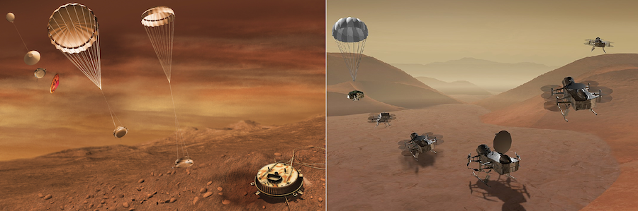
Figure 1: Artists’ depictions of the Huygens probe (left) compared to Dragonfly (right) arriving on Titan. [Left: ESA/C. Carreau; right: NASA]

Descending onto Titan

Like any lander mission to a planetary surface, safety is the first consideration for narrowing down landing sites. In the mid-2030s — the arrival time planned for the mission — Titan’s northern hemisphere will be pointed away from Earth and the Sun. Since Dragonfly relies on a direct line of sight for communication, and NASA requires active tracking during the spacecraft’s entry, descent, and landing phase, this mission therefore can’t be sent to the intriguing methane seas at Titan’s north pole. Instead, dune fields near the equator make for yet another enigmatic target on Titan, where the composition of the organic sand and its origin are not yet well understood.

To avoid the need for additional propellant, the spacecraft will sneak up behind Titan (rather than hitting head-on) and use an aeroshell to slow down in Titan’s thick atmosphere. Assuming that Dragonfly enters at the same 65-degree angle as the Huygens probe, these constraints further narrow down potential landing sites on Titan to a donut-shaped “viable target region” (see Figure 2). From this region, the team was soon drawn to a large impact crater that may provide a variety of interesting terrains for study.

A grayscale projection of Titan's surface. The equatorial region is spanned by several large dark patches. Several lakes and seas, known as maria, dot the north pole. Yellow annotations indicate the reasons for considering or not considering various locations for a landing site. Lack of daylight excludes most areas with longitudes between -120 and 60. The steepness or shallowness of the spacecraft's entry further restricts options to a donut-shaped region centered on 110 degrees longitude and 10 degrees latitude.

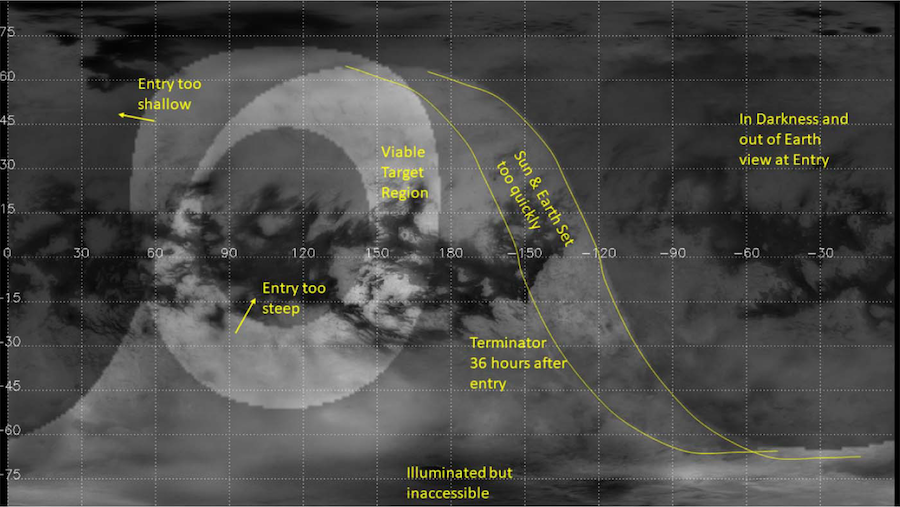
Figure 2: A map of Titan from the Cassini spacecraft’s Imaging Science Subsystem with annotations concerning various considerations for landing. Dragonfly’s proposed landing site, near Selk Crater, is at 3.7°N, 161.8°E. [Lorenz et al. 2021]

Preparing for Landing

The chosen location on Titan, Selk Crater, makes for an interesting study region, in part because of the fascinating chemical reactions possible there. Though Titan is extremely cold and icy, it is wrapped in a haze of organic molecules (long chains of carbon, hydrogen, and nitrogen) that have likely reacted to form the basic building blocks of life. Following the extreme heat of an impact, ice melted into liquid water would have created a fascinating organic soup that may have even been briefly habitable before freezing back into place. Besides the astrobiological potential, the crater and nearby dunes have obvious geological interest. For example, ongoing erosion by winds and methane rains has likely degraded the crater rim.

Despite the sometimes sparse data available for Titan, Selk Crater also has the benefit of having relatively good coverage for mission planning, thanks to several flybys during the Cassini mission. Visible and near-infrared images indicate the chemical composition of the surface based on the brightness of reflections at different wavelengths, but often the highest-resolution data for studying morphology comes from radar images (see Figure 3). Some limited topographic data further suggest that the region has relatively minor slopes, rather than steep mountains that could be hazardous to the mission.

To study the region around Selk Crater, the team divided the area into a grid with quarter-degree (~10 km or ~6 mi wide) cells. Making a map for each of the three main Cassini datasets (visible light, infrared, and radar), each cell is given a classification, indicating, for example, whether that cell contains dunes, less-certain dunes, ice-rich impact ejecta, or insufficient data, among other classes similar to those used in previous maps. These grid cells can then be used to define mission plans, including a specific landing location. Based on simulations of the atmosphere and its winds, the team defined a 149 by 72 km (93 by 45 mi) landing ellipse south of the crater, within which the probe has a 99% chance of landing.

Three images of Selk Crater. Left: A black and white image showing the bright crater rim and ejecta blanket extending down and to the right against the dark background. Center: A representative-color image of the same region in slightly greater detail. Right: A zoomed-in image of the same region with the landing ellipse marked below the crater.

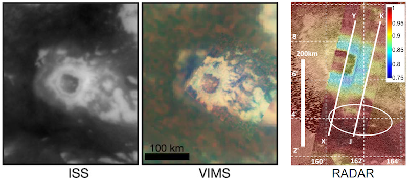
Figure 3: Selk Crater seen in various datasets. Left and center images with black borders are from the near-visible-wavelength ISS (Imaging Science Subsystem, left) and infrared-wavelength VIMS (Visual and Infrared Mapping Spectrometer, center). Zoomed in somewhat closer, the radar mosaic (right) also shows the location of two topographic profiles (XY and JK) and the landing ellipse in white, with colors representing the microwave emissivity. [Adapted from Lorenz et al. 2021]

Setting Your Expectations

In addition to the available data, scientists can also make inferences about the surface conditions by drawing analogies to similar geologic features on Earth (see Figure 4). The “interdune” area between dunes is expected to be flat and safe, so Dragonfly won’t tip over! Since Titan’s dunes are expected to have the same morphology as dunes on Earth, there should be wide sections of each dune that are shallow in slope so that Dragonfly can safely take samples of the sand. Ultimately, if things go well among the dunes, the craft will progressively work its way north into the ejecta blanket and Selk’s interior. Terrestrial analogs for Selk similarly give researchers confidence that the interior of the crater will be relatively flat and hospitable to Dragonfly.

With several years remaining before launch, further changes to the plan might occur, but the team expects that any remaining changes to the landing ellipse will be relatively minor. Ongoing studies will dig deeper into the Cassini–Huygens data in preparation for this ambitious mission. Although Dragonfly’s launch was delayed to 2027 (with arrival at Titan in 2034), it looks like a visit to Selk Crater will certainly be worth the wait!

Top left: Two long, straight, radar-bright dunes extend from the upper left to the lower right of the image. Bottom left: A sinuous dune with flat sand to either side. Right: A flat area with winding streams lies in front of a crater rim.

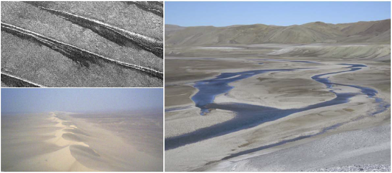
Figure 4: Terrestrial analogs for the landing site on Titan. Linear dunes in Egypt seen from above in radar (top left) and near the ground (bottom left) are likely very similar to those on Titan. The Haughton impact structure in northern Canada (right) is likely similar to Selk, with a flat area inside the crater rim. [Adapted from Lorenz et al. 2021]

Original astrobite edited by Haley Wahl.

About the author, Anthony Maue:

Anthony is a PhD candidate at Northern Arizona University in Flagstaff studying planetary geology. In particular, his research focuses on Titan’s fluvial processes through analyses of Cassini radar data, laboratory experiments, and terrestrial field analog studies. He is also one half of the planetary science podcast Out of the Silent Planet. Back on Earth, Anthony enjoys skiing, cycling, running, music, and film.

illustration of a brown dwarf

Editor’s note: Astrobites is a graduate-student-run organization that digests astrophysical literature for undergraduate students. As part of the partnership between the AAS and astrobites, we occasionally repost astrobites content here at AAS Nova. We hope you enjoy this post from astrobites; the original can be viewed at astrobites.org.

Title: Ross 19B: An Extremely Cold Companion Discovered via the Backyard Worlds: Planet 9 Citizen Science Project
Authors: Adam C. Schneider et al.
First Author’s Institution: United States Naval Observatory, Flagstaff Station
Status: Published in ApJ

Typically thought of as stars that didn’t quite make it, brown dwarfs are a class of object without enough mass to undergo hydrogen fusion like other main-sequence stars, but heavy enough to fuse deuterium, differentiating them from their gas giant planet cousins. With faint spectra and complex evolutionary tracks, uncovering the properties of a brown dwarf can be much more challenging than your typical star or planet, particularly if the brown dwarf does not have a companion to help determine its age and mass.

However, ever the classifiers, astronomers often separate brown dwarfs into one of three spectral types — L, T, and Y — based on their temperature. The coldest and newest category of brown dwarfs, the Y dwarfs, have so far proven especially hard to study. Out of the only 25 known Y dwarfs, only one, WD0806-661B, has a stellar-mass companion. Since the presence of companions enables the use of techniques like radial velocities to refine system parameters, this means that the ranks of the coldest brown dwarfs are severely lacking in well-constrained masses and ages.

Enter Stage Left: CWISE J021903.84+352112.2

Meet Ross 19B, the newest discovery of the Backyard Worlds: Planet 9 citizen science project. As its “B” designation suggests, Ross 19B is a companion to the nearby M-type star Ross 19A, and it was first identified as a candidate brown dwarf (and labelled CWISE J021903.84+352112.2) by citizen scientists Samuel Goodman, Léopold Gramaize, Austin Rothermich, and Hunter Brooks. By searching through sets of images from NASA’s Wide-field Infrared Survey Explorer (WISE) mission, the citizen scientists were able to identify that Ross 19A and the candidate object had similar proper motions — the way in which nearby objects appear to move across the sky with respect to more distant stars, which remain comparatively constant — as seen in Figure 1. This kind of co-movement suggests that Ross 19A and the candidate are likely physically associated, and they could be binary companions to each other.

Two negative-color images from the WISE mission arrayed vertically, showing black stars and other objects against a tan background. The top image is labeled 2010 and the bottom image is labeled 2019. Each image has two pairs of blue and white circles, showing the positions of Ross 19A and Ross 19B, as well as a square with a zoomed in image of Ross 19B.

Figure 1: Images from the WISE mission demonstrating the similar proper motion of the M-type star Ross 19A and the candidate brown dwarf, taken in 2010 (top panel) and 2019 (bottom panel). Ross 19A (labelled as Ross 19) is seen in the top right-hand corner of each panel, while the candidate object that would become Ross 19B (labelled as CWISE J021903.84+352112.2) is in the bottom left-hand corner. To highlight the proper motion of each object, the white circles in both panels indicate their positions in 2010, while the blue circles do the same for 2019. In both panels, inserts show a zoom-in of the location of Ross 19B, seen as a small brown dot. [Schneider et al. 2021]

To confirm that the candidate object was indeed a companion to Ross 19A and not aligned with it by chance, the authors estimated the probability that the two objects are co-moving using the CoMover code. CoMover makes use of the BANYAN Σ software’s ability to determine how well the position, proper motion, and parallax of an object match with the galactic coordinates and velocities of nearby groups such as stellar associations. With the new CoMover tool, the authors find a 100% probability that Ross 19A and the candidate are physically associated, and the team officially designates the new brown dwarf as Ross 19B.

What Makes Ross 19B So Special?

With the available photometry and the known distance to the Ross 19 system, the spectral type of Ross 19B can be found by calculating its J-band magnitude and converting this to a spectral classification. Ross 19B was found to have a J-band magnitude of ~19.6, corresponding to the boundary between T and Y dwarfs, and a temperature of around 500K. As seen in Figure 2, this makes Ross 19B the coldest known brown dwarf companion within 20 parsecs of the Sun, with the exception of the only known Y-dwarf companion, WD0806-661B.

Plot showing the J-band magnitudes and spectral types of brown dwarfs within 20 parsecs of the Sun. The x-axis (spectral type) ranges from L0 to just beyond Y0. The y-axis (J-band magnitude) ranges from 24 to 10. The placement of the gray rectangle indicating the J-band magnitude of Ross 19B, places it at a spectral type around Y0.

Figure 2: Plot showing the J-band magnitudes and spectral types of brown dwarfs within 20 parsecs of the Sun, with cooler objects towards the right and brighter objects towards the top. Brown dwarfs which have companions are highlighted by the blue circles, while brown dwarfs without companions are shown by the black points. The J-band magnitude of Ross 19B and its error bars are shown by the grey region. With a spectral type near the T/Y boundary, Ross 19B is likely the coldest local brown dwarf companion, with the exception of the Y dwarf WD 0806-661B. [Adapted from Schneider et al.]

Using Ross 19B’s companion to their advantage, the authors are also able to make estimates about the physical parameters of the system. Ross 19A is a low-metallicity star with no signs of activity such as stellar flares, indicating that the star is several billion years old. Using this estimate along with the spectral type of Ross 19B, evolutionary models suggest that Ross 19B could have a mass around 15–40 times that of Jupiter, towards the lower end of typical brown dwarf masses. Meanwhile, at over 11,000 au, the separation of Ross 19A and B makes the system one of the widest found to date!

Given all these factors, Ross 19B provides a fascinating new case study, helping us to expand our understanding of brown dwarfs into colder and wider territories.

Original Astrobite edited by Pratik Gandhi.

About the author, Lili Alderson:

Lili Alderson is a first year PhD student at the University of Bristol studying exoplanet atmospheres with space-based telescopes. She spent her undergrad at the University of Southampton with a year in research at the Center for Astrophysics | Harvard-Smithsonian. When not thinking about exoplanets, Lili enjoys ballet, film and baking.

Image of a background quasar that has been smeared into a ring, with 4 bright dots visible within the ring. A foreground galaxy can be seen in the ring's center.

Editor’s note: Astrobites is a graduate-student-run organization that digests astrophysical literature for undergraduate students. As part of the partnership between the AAS and astrobites, we occasionally repost astrobites content here at AAS Nova. We hope you enjoy this post from astrobites; the original can be viewed at astrobites.org.

Title: ALMA Observations of the Sub-kpc Structure of the Host Galaxy of a z = 6.5 Lensed Quasar: A Rotationally-Supported Hyper-Starburst System at the Epoch of Reionization
Authors: Minghao Yue et al.
First Author’s Institution: Steward Observatory, University of Arizona
Status: Published in ApJ

The party starts at dawn, and you all are invited! You’ll be surrounded by new, up-and-coming stars and a big fireworks show! There’s even a house of mirrors, where you can see a distorted, magnified version of yourself. Be careful of the action in the very center — it’s bright and shiny, but if you get too close, you could get ejected from the party entirely. Looking back, your view of the party might get a little warped, but it will surely be a bright point. Oh, and it’s hosted by a luminous quasar (z = 6.5) that is powered by a supermassive black hole — you can’t miss it!

Into the Cosmic House of Mirrors

In today’s paper, the authors target a gravitationally lensed quasar and its host galaxy in the early universe, the first of its kind to be observed so far back in spacetime (during cosmic dawn). Gravitational lensing occurs when mass along the observer’s line of sight distorts light before it reaches the observer, turning the universe into a sort of cosmic house of mirrors. During the process, some clump of mass (in this case, another galaxy) in the foreground magnifies and warps the light — a consequence of general relativity — coming from the background object (here, the quasar and its host galaxy). To get a sense of how this works, see Figure 1 below, or check out the iOS app GravLens3!

Schematic diagram illustrating how gravitational lensing works.

Figure 1: Diagram demonstrating gravitational lensing. Light from the more distant quasar is intercepted by a massive foreground galaxy, causing the light to be bent and magnified. The resulting image seen by the telescope shows the foreground galaxy surrounded by multiple images of the lensed quasar. [NASA/ESA/D. Player (STScI)]

This lensing is like having an extra, natural telescope amplifying the signal and providing a higher resolution image. For this dataset, the galaxy’s light is boosted by about 4 times, and stretched out enough to resolve structure on small scales. But the amplification doesn’t come for free — the lensing also manipulates the image from the background source. While the lensed object is actually a single blob, the lensed image we get is stretched out and appears multiple times, depending on how the mass of the foreground lens is distributed and positioned with respect to the background lensed object.

Hyper-Starbursting and Supersized

Quasars, some of the brightest and most extreme objects in the universe, are found in galaxies during a temporary mega-bright phase (see this astrobite for more about how they grow). During this phase, their central supermassive black holes vigorously funnel in material, building a disk of hot, luminous material around it and ejecting material via energetic jets. While quasars are bright and easy to detect, the galaxies that host and fuel them are often hidden behind the shining quasar in their active centers. However, if we can peer behind the quasar and target the gas and dust in the host galaxy, we can better understand the nature and origin of the galaxy–quasar system.

Today’s authors use millimeter wavelength observations from the Atacama Large Millimeter/submillimeter Array (ALMA) to measure the host galaxy’s dust and [CII] emission. [CII] is a molecular emission line that is commonly used to trace the motions and content of gas, the main fuel source for luminous galaxies. These observations provide clues about the structure, motions, and star formation activity within the host galaxy. After building a model of the lens to disentangle the multiple images into the original single source, the authors were able to confirm their previous lens model based on HST data (see the group’s earlier paper), and model the new ALMA data.

Based on their reconstruction of the background host galaxy (see Figure 2), the light profile looks like your everyday disk galaxy, and the kinematic tracers show a smooth velocity structure. These clues together suggest that the host galaxy is a regular, rotating disk, like a vinyl spinning around on a record player. However, the dynamics are a bit more complicated, as the galaxy doesn’t appear to be symmetric along its axes, nor does it seem to be a thin disk — so, not quite a vinyl on a record player. It could just be clumpy, but more likely it has a thick geometry and is more spheroidal than disky. Higher resolution observations are needed to better understand the complex kinematics going on here, which are a common feature of high redshift quasars.

Two plots describing velocity structure of the quasar's galactic host, first as a Dec vs. RA plot with velocity represented by colors, and then as a velocity vs. position plot.

Figure 2: Left: velocity structure of the host galaxy, which shows a smooth rotation with blue moving towards and red moving away from the observer. The red curves trace the caustic, which describes the gravitational lensing and marks the curve of highest magnification. The black line corresponds to the right panel. Right: breakdown of the position and velocity across the galaxy. This also shows generally smooth rotation, with a minor irregular feature in the yellow box (region corresponding to black dots in the left panel). [Yue et al. 2021]

The kinematics also provide key measurements that can be used to estimate properties of the galaxy’s supermassive black hole. In the local universe, the mass of a central supermassive black hole and the mass of its host galaxy follow a simple positive relation. In this paper, the authors describe their galaxy’s black hole as oversized, as it’s relatively large compared to the host galaxy. This has been found for other similar distant quasars, and suggests a fundamental difference in the coevolution of black holes within quasar systems and their host galaxies at early times.

A Case Study for the Extreme

This system is the farthest lensed quasar in the universe (redshift z = 6.5) discovered so far, among the very first stars and galaxies (to learn about the most distant quasar currently known, which is non-lensed, check out this astrobite.) It’s a pretty intense system, with an extreme star formation rate and efficiency, and an overly massive black hole in the middle — definitely a real rager of a party. Yet these extreme characteristics are not necessarily unique, and they have been observed for the small sample of (non-lensed) quasars at cosmic dawn with ALMA. What makes this galaxy in particular so special is the fact that it’s gravitationally lensed, allowing for observations with much higher detail and signal. Moreover, the authors refer to this quasar as a case study for probing the nature, origin, and structures of quasars at cosmic dawn, and for understanding how supermassive black holes and their host galaxies co-evolve. Looking ahead to future studies, the authors hope to use higher resolution data to measure the influence of the central black hole more directly, confirm the geometry of the galaxy, and more precisely map its velocity field. Back into the cosmic house of mirrors at the party at dawn!

Original astrobite edited by James Negus.

About the author, Olivia Cooper:

I’m a first year grad student at UT Austin studying the obscured early universe, specifically the formation and evolution of dusty star-forming galaxies. I recently graduated from Smith College where I studied astrophysics and climate change communication. Besides doing science with pretty pictures of distant galaxies, I also like driving to the middle of nowhere to take pretty pictures of our own galaxy!

Illustration of a faint, red gas giant planet orbited by a dark, rocky body.

Editor’s note: Astrobites is a graduate-student-run organization that digests astrophysical literature for undergraduate students. As part of the partnership between the AAS and astrobites, we occasionally repost astrobites content here at AAS Nova. We hope you enjoy this post from astrobites; the original can be viewed at astrobites.org.

Title: On the Detection of Exomoons Transiting Isolated Planetary-Mass Objects
Authors: Mary Anne Limbach et al.
First Author’s Institution: Texas A&M University
Status: Published in ApJ

When faced with the sheer beauty of shimmering stars emblazoned across a night’s sky, it’s hard not to imagine that there are innumerable other worlds out there — entire planets teeming with alien life, or ruins of once-great civilisations. Until recent decades, such imagination was confined to the realm of science fiction, but in 1992 came the first detection of an exoplanet: a planet outside our solar system.

Illustration of a rocky body next to a gas giant planet, with a distant star and another small body in the background.

Artist’s depiction of an Earth-like exomoon orbiting a gas-giant planet. [NASA/JPL-Caltech]

The study of exoplanets provides important insights into the physics that govern the formation and evolution of planetary systems — in addition to raising many philosophical questions — but exoplanets are notoriously difficult to detect. The primary method of detection relies on measuring the dimming of a parent star during a planetary transit. Even more difficult to detect are exomoons: moons orbiting exoplanets. They are almost impossible to image directly due to the glare of the host star and, due to their smaller size, harder to detect via transit photometry. However, exomoons are believed to be at least as common as exoplanets. The authors of today’s paper point to a source where exomoons may be more easily detected: isolated planetary-mass objects (IPMOs), also known as rogue or nomadic planets.

Sunless Skies

Rogue planets are not bound to a planetary system. Instead, they roam free throughout the galaxy, bathed in darkness and lit by no sun. This makes it much easier to detect exomoons that orbit IPMOs compared to those orbiting ordinary exoplanets. The authors estimate that for over half of all known IPMOs, the sensitivity of the upcoming James Webb Space Telescope (JWST) is enough to detect the presence of an exomoon with similar characteristics to Jupiter’s moon Ganymede. Before planning an exomoon hunt, one must first consider observational constraints. One of the most important is the probability of observing a transit in the first place. Simulations have demonstrated that the formation of moons is common — with at least one large moon forming in roughly 80% of planetary systems — and that these moons often resemble the Galilean moons with respect to their sizes and orbital configurations.

Moonlight Sonata

It is therefore sensible to model probabilities based on moons in our own solar system, such as those orbiting the gas giants. The authors first model the transit probabilities for the solar system gas giant moons — that is, they find the probabilities that a moon will cross the face of the gas giant — with respect to some randomly oriented observer located outside the solar system.

Figure 1 shows the probabilities of observing at least one transit in some system of planets, as well as the observed transit depths. In this case, the transit depth refers to the fractional dip in the light curve of a planet as it is transited by its moon. Supposing that we observed 10 planets with moons, the probability of observing a transit of an Io-like moon is about 85%. For a Europa-like moon, the transit probability drops to 70%, while transits of Mercury-like and Jupiter-like moons are much rarer, at 10% and less than 1% probability respectively.

two side by side plots show transit probability vs. number of objects and transit depth vs. orbital period

Figure 1: Left: Probability of observing at least one transit as a function of the number of objects (exoplanets) in the sample. The curves represent different solar system objects. Right: Percentage transit depth as a function of orbital period for various planets and moons in our solar system. [Limbach et al. 2021]

Figure 2 shows the orbital periods and durations of possible transits as functions of orbital radius. In general, the closer the exomoon is to the exoplanet, the more likely it is that we’ll observe an exomoon transit. Based on Figure 2, the authors suggest that most exomoons will have a transit probability of 10 to 20%, and that they will likely be detected within a minimum of 50 hours of observation.

two side by side plots show orbital period and transit duration vs. semimajor axis

Figure 2: Left: Orbital period of an exomoon versus its orbital distance (in both astronomical units and kilometres). The curves denote super-Jupiter mass IPMOs with transit probabilities listed. The Roche limit is the closest the moon can orbit the planet. Right: Similar to the left panel, but with transit duration on the vertical axis. [Limbach et al. 2021]

Roguelike Exomoons

The main advantage of looking for moons around IPMOs is that high-contrast and high-resolution imaging is not needed; there is no interference from a nearby host star to drown out any signal. Instead, current ground telescopes can observe IPMOs with very high precision. Next-generation space-based telescopes, such as the imminent JWST, will further improve this precision by an order of magnitude.

Figure 3 shows the radius of moons orbiting Jupiter-mass exoplanets versus the photometric precision required to accurately detect their transit. Current high-contrast imaging of stellar-bound exoplanets can only detect moons at least as big as Neptune. With IPMOs, ground-based imaging allows for the detection of Earth-sized moons. With the JWST, it will be possible to detect Ganymede-sized moons, and even moons down to the size of Titan or Io! The authors calculate that the JWST will be able to detect Ganymede-sized moons around over half of all known IPMOs.

plot of moon radius vs. photometric precision for a 5 sigma detection

Figure 3: Exomoon radius (in units of Earth radii) versus the photometric precision required for an accurate transit detection (logarithmic scale). Smaller precision values correspond to higher resolutions. The solid and dotted curves denote Jupiter mass and 1.5 x Jupiter mass IMPOs, with the shapes corresponding to the sizes of orbiting moons. Vertical lines denote the sensitivity limits of current/future observations. [Adapted from Limbach et al. 2021]

Sic Mundus Creatus Est

Exomoons are believed to be just as common as exoplanets, with at least one large moon forming around approximately 80% of simulated planets. Rogue exoplanets can be observed with a higher photometric precision since there is no glare/interference from a nearby host star. Moon–planet transits are also relatively common, and more than half of all known IPMOs are bright enough to allow for the detection of a Ganymede-sized moon. However, the authors propose a minimum observing time of 50 hours, which adds up to nearly 17 weeks of combined observing time for the 57 known IPMOs. The authors note that IPMO exomoons are among the most accessible candidates for detecting habitable worlds (in this case, the moon is warmed by tidal heating rather than by a star). Potentially habitable IPMO exomoons would not only lend insight into the processes governing planet formation, but could also offer a window into the conditions of the primordial Earth, thus allowing us to place a timescale on the development of life itself.

Original astrobite edited by Ryan Golant.

About the author, Mitchell Kavanagh:

Mitchell is a PhD student in astrophysics at the University of Western Australia. His research is focused on the applications of machine learning to the study of galaxy formation and evolution. Outside of research, he is an avid bookworm and enjoys gaming, languages and code jams.

pulsar

Editor’s note: Astrobites is a graduate-student-run organization that digests astrophysical literature for undergraduate students. As part of the partnership between the AAS and astrobites, we occasionally repost astrobites content here at AAS Nova. We hope you enjoy this post from astrobites; the original can be viewed at astrobites.org.

Title: The Location of Young Pulsar PSR J0837−2454: Galactic Halo or Local Supernova Remnant?
Authors: Nihan Pol et al.
First Author’s Institution: West Virginia University; Vanderbilt University
Status: Published in ApJ

In 1967, a graduate student named Jocelyn Bell Burnell discovered the first pulsar, opening a window into a universe teeming with many wild and wonderful varieties of these extreme objects. Pulsars are fast-spinning neutron stars with powerful magnetic fields, emitting beams of radio waves. They give rise to many interesting phenomena: some pulsars cannibalize companion stars, others emit pulses of high-energy gamma rays, and still others exhibit sudden changes in their rotation period.

Despite this diversity, pulsar astronomers have managed to establish some typical properties of pulsars. For example, pulsars — especially very young pulsars — are rarely found far from the plane of the Milky Way. The stars that form them usually live in the galactic disk, and many pulsars simply don’t have enough time to move away. Today’s paper, however, focuses on a pulsar that seems to be much farther from the galactic plane than we should expect. What could be going on?

The Paradoxical Pulsar

This particular pulsar, designated J0837–2454, was discovered in 2011 using the Parkes Radio Telescope. However, it took six more years to produce enough data to adequately constrain its properties. The authors found that the pulsar was young, estimating its age to be a mere 28,600 years, with a reasonable rotation period and magnetic field. What made it stand out like a sore thumb was its dispersion measure, or DM. The dispersion measure describes how many free electrons lie between us and the pulsar, so it acts as a sort of distance proxy: if you know the DM, the location of the pulsar in the sky, and how the galaxy’s electrons are distributed, you can calculate its distance from us.

The astronomers picked two widely used models of the Milky Way’s electron density, derived from, among other things, measurements of dispersion measures and distances to known pulsars. One, the NE2001 model, predicted that J0837–2454 should lie 6.3 kpc (a bit over 20,000 light-years) from Earth, placing it a whopping 1.1 kpc above the galactic plane — much higher than any pulsar of comparable age. The other, the YMW model, predicted that it should lie beyond the galactic disk. Both would be a surprising result, so the authors considered other means of estimating the distance to the pulsar.

plot of vertical distance from the galactic plane vs. planar distance from galactic center for known pulsars

Figure 1: Most pulsars (shown in red) lie close to the galactic plane, and previously known pulsars less than 50,000 years old (in green) tend to be even closer. According to a standard model of the Milky Way’s electron distribution, PSR J0837-2454 (marked with a blue asterisk) appears to lie at least twice as far away as any other known pulsar of comparable age. [Pol et al. 2021]

Getting a Second Opinion — and a Third

Many young pulsars are associated with supernova remnants (SNRs), so it made sense to see if there was one near J0837–2454. The group used the Australia Telescope Compact Array (ATCA) to search for radio emission from a remnant, supplementing their observations with archival images from the radio Galactic and Extra-galactic All-sky MWA Survey (GLEAM) and the Southern Hα Sky Survey (SHASSA).

The ATCA observations were unable to detect any SNR-like emission, but the GLEAM images showed a faint structure near the pulsar, which might represent an SNR. Assuming this is actually an SNR associated with the pulsar, this structure could provide an independent estimate of the distance to J0837-2454: models of SNR evolution could estimate its physical size and compare that to its angular size, thus yielding the distance to the source. Using this method, the authors found a distance of only 0.9 kpc from Earth, placing the structure — and the pulsar, if the structure is, indeed, an associated SNR — at a more reasonable offset from the plane.

image showing the location of the pulsar, remnant, and nearby second pulsar

Figure 2: Stacked images from the Galactic and Extra-galactic All-sky MWA Survey (GLEAM) show an excess of radio emission in a round region overlapping with PSR J0837–2454, marked by a red cross. This excess has been interpreted as a possible supernova remnant associated with the pulsar. A second nearby pulsar, PSR J0838–2621, is marked by a purple cross and is believed to be unassociated with the pulsar and the candidate supernova remnant. [Pol et al. 2021]

The SHASSA data also provided another way out of the quandary. The images showed a diffuse Hα structure near the position of the pulsar, distinct from the radio emission detected by GLEAM. The authors suggested that this emission was unrelated to the pulsar, but instead lay between it and Earth. This could be contributing to the surprisingly high dispersion measure. If this is true, the SHASSA results would place the pulsar as close as 0.2 kpc from us and close to the plane.

Tying Up Loose Ends

There are still several issues to consider. Assuming the distance derived from the NE2001 model is correct, how could the pulsar have traveled so far from the disk? To have traveled 1.1 kpc in 28,600 years would require the pulsar to be moving unreasonably fast. However, this rests on the assumption that the pulsar was born within the disk; it’s possible that it actually formed much closer to its present position. The massive progenitor could have been a runaway star, propelled away by a companion star going supernova. One way of confirming or refuting this scenario would be to measure the velocity of the pulsar out of the plane — not an easy task, but not impossible.

This still leaves an obvious problem: if NE2001 distance estimate is correct, why didn’t ATCA detect a supernova remnant? It’s possible that the structure detected by GLEAM is completely unrelated to the pulsar, and that the real SNR is simply too faint. If the circumstellar medium around the pulsar is too diffuse, or the magnetic field is too weak, the remnant would be unable to generate strong enough synchrotron emission at radio frequencies for it to be detectable by ATCA. A combination of the two seems to be a feasible explanation. As next-generation radio telescopes like the Square Kilometre Array come online, maybe we can find the final pieces of this pulsar puzzle.

Author’s note: While Nihan Pol, Sarah Burke-Spolaor and Harsha Blumer are or have been part of my department, I was not involved with this research.

Original astrobite edited by Sabina Sagynbayeva.

About the author, Graham Doskoch:

I’m a first-year graduate student at West Virginia University, pursuing a PhD in radio astronomy. My focus is on neutron stars and pulsar timing, a method of detecting gravitational waves by monitoring arrays of pulsars over the course of many years. I’m an associate member of NANOGrav, and I’m starting to help with their ongoing timing efforts. I love running, hiking, reading, and just enjoying nature.

Aerial image of a large rectangular structure surrounded by a circle in the landscape. Circular tanks are visible to the right of the structure.

Editor’s note: Astrobites is a graduate-student-run organization that digests astrophysical literature for undergraduate students. As part of the partnership between the AAS and astrobites, we occasionally repost astrobites content here at AAS Nova. We hope you enjoy this post from astrobites; the original can be viewed at astrobites.org.

Title: Discovery of the Ultra-High Energy Gamma-Ray Source LHAASO J2108+5157
Authors: Zhen Cao, F. A. Aharonian, Q. An, et al. (the LHAASO collaboration)
First Author’s Institution: Institute of High Energy Physics, Chinese Academy of Sciences, China
Status: Published in ApJL

The Hunt for PeVatrons

composite image of a complex-structure spherical bubble of emitting gas of different colors

Figure 1: An image of the supernova remnant Cassiopeia A from NASA’s Chandra X-ray Observatory.  [NASA/CXC/SAO]

What are our galaxy’s most energetic and extreme particle accelerators? Could it be supernova remnants, the remains of the violent death of a massive star? Or might it be the nebulae that form around pulsars, rapidly rotating and highly magnetized neutron stars? Perhaps surprisingly, this is still an open question in high-energy astrophysics and the list of possible suspects is much larger than just those mentioned above.

However, we know that these particle accelerators exist. We know this because we are constantly being bombarded by high-energy cosmic rays — protons or heavier atomic nuclei that are traveling at nearly the speed of light. Now, over 100 years since Austrian physicist Victor Hess discovered cosmic rays by taking an electroscope on a hot air balloon flight, we still don’t know what astrophysical objects produce the highest energy cosmic rays. Some of these cosmic rays have an energy over 1 Petaelectronvolt (PeV = 1015 electronvolts), comparable to that of a mosquito’s kinetic energy, but packed into a single proton.

The cosmic objects responsible for producing PeV cosmic rays are so called “PeVatrons,” and pinpointing these sources is no small feat. However, as these cosmic rays are so energetic, they are akin to a bull in a china shop, and they frequently collide with gas or material that surround the PeVatrons. These interactions produce gamma rays that carry about 10% of the energy of the initial cosmic ray. Thus, finding gamma rays with energy of about one tenth of a PeV (100 TeV) is a smoking gun for a PeVatron.

Photo of a series of circular tanks located in the ground on the side of a large rectangular structure.

Figure 2: Another aerial view of the Large High Altitude Air Shower Observatory (LHAASO). The cylindrical tanks help detect muons, which can be used to distinguish gamma rays from unrelated cosmic rays. [Liu Kun/Xinhua/Alamy]

This is exactly what the authors of today’s paper set out to accomplish. The paper discusses using a detector that is still being constructed in Sichuan, China, the Large High Altitude Air Shower Observatory (LHAASO). LHAASO consists of many small detectors spread out over an area greater than a square kilometer. When a high-energy gamma ray from a PeVatron enters the atmosphere, it can collide with a particle in the atmosphere and create a very large shower of subatomic particles. The array of detectors on the ground can detect these particles and reconstruct the shower to infer properties about the initial gamma ray. A picture of part of LHAASO is shown in Figure 2.

Although LHAASO is not even done with construction, its immense size already makes it an extremely efficient gamma-ray detector. To date, LHAASO has detected 12 sources of these ultra-high-energy (UHE) gamma rays, and has even detected the highest energy photon from an astrophysical source yet found. While all of these sources provide a wealth of information on galactic PeVatrons, one of the objects — LHAASO J2108+5157, the focus of today’s paper — is particularly interesting because of its mysterious origins.

Figure 3 shows the detection of this object at energies between 25 TeV and 100 TeV, as well as for higher energies. The source is significantly detected in both of these energy ranges. However, what is strange is that while all of the other 12 sources have been detected by other telescopes in the “very-high-energy” band (around 1 TeV or so, which is high energy but still below the energy detection limit of LHAASO), this is the only object that is significantly detected at higher energies but does not have a counterpart at 1 TeV.

side by side 2D heatmaps showing bright sources in the middle of each

Figure 3: Significance map in the region around the newly detected source, LHAASO J2108+5157. The left shows gamma rays with energies between 25 TeV and 100 TeV and the right shows gamma rays above 100 TeV. The cross denotes the best-fit location of the source and the red circles show an approximate uncertainty on this location. The white circles show the average directional uncertainty for individual gamma-ray events. [Cao et al. 2021]

The authors spend some time in the paper exploring what could be causing this UHE gamma-ray signal by looking for counterparts in other wavelengths, even if there aren’t counterparts detected in the 1 TeV gamma-ray band. While many of the other 12 sources were coincident with supernova remnants (SNRs) or pulsar wind nebulae (PWNe), no objects like this lie anywhere close to LHAASO J2108+5157.

However, the authors note that this object is spatially coincident with a molecular cloud. Distinguishing between the molecular cloud scenario and the SNR or PWN scenario is crucial, as the presence of a molecular cloud could indicate this source is accelerating protons to these high energies. In the case of SNRs or PWNe, it is only believed that these objects might accelerate electrons (not protons) to high energies. The distinction between these two acceleration scenarios has dramatic implications for the spectra of cosmic rays. Figure 4 explores these two options by modeling what proton acceleration might predict versus electron acceleration. Although both models are consistent with the data, the authors believe the presence of a catalogued molecular cloud is promising for the proton scenario. Hopefully, future observations will be able to distinguish between these two cases.

SED over many decades in energy. Data points are consistent with lines that show various model predictions

Figure 4: LHAASO data (red) compared to various models that would predict gamma-ray emission. The solid red line shows a model based on the acceleration of protons (hadronic) and the dashed green is based on photons scattering off of accelerated electrons (leptonic, labeled IC CMB in the plot). Although the data are consistent with both, distinguishing between these models is crucial for finding the sources of the highest energy cosmic rays. [Cao et al. 2021]

With the first dozen detected sources at these ultra-high energies, there is already a vast amount of insight that has been gained on the nature of PeVatrons. However, as LHAASO is still being constructed and will only improve and continue to take more data, the future of ultra-high energy gamma-ray astronomy will undoubtedly be bright.

Original astrobite edited by Katy Proctor.

About the author, Alex Pizzuto:

Alex is a PhD candidate at the Wisconsin IceCube Particle Astrophysics Center at the University of Wisconsin-Madison. His work focuses on developing methods to locate the Universe’s most extreme cosmic accelerators by searching for the neutrinos that come from them. Alex is also passionate about local science outreach events in Madison, and enjoys hiking, cooking, and playing music when he is not debugging his code.

An artist's depiction of a Thorne-Zytkow object. The image shows a blue-ish/white sphere representing the neutron star core inside of a larger reddish-orange sphere, representing the red supergiant.

Editor’s note: Astrobites is a graduate-student-run organization that digests astrophysical literature for undergraduate students. As part of the partnership between the AAS and astrobites, we occasionally repost astrobites content here at AAS Nova. We hope you enjoy this post from astrobites; the original can be viewed at astrobites.org.

Title: Prospects for Multimessenger Observations of Thorne-Żytkow Objects
Authors: Lindsay DeMarchi, J. R. Sanders, and Emily M. Levesque
First Author’s Institution: Northwestern University
Status: Published in ApJ

The universe is full of different types of stars, including big ones called red giants. But what if some of those red giants are hiding another star inside them?

Two Stars for the Price of One?

illustration of a large red star surrounded by spherical shells of mass

Artist’s illustration of a red giant star expelling mass at the end of its life. [JAXA]

A Thorne-Żytkow object (TZO) is a very special type of hybrid object that consists of two stars: a red giant (or supergiant) and a neutron star that lies at the core of the red giant. One way a TZO could be created is from the evolution of a close binary of two massive stars (> 8 solar masses) orbiting each other. Once the more massive star from the pair reaches the end of its lifetime, it will go supernova and leave behind a small, dense neutron star. This process could cause the neutron star and the remaining massive star to inspiral, allowing the red giant to swallow the tiny, but dense, neutron star — perhaps the most epic fit of celestial sibling jealousy!

The Challenges of Detecting a TZO

Though TZOs were first proposed in 1977, they remain extremely hard to detect and have never been observationally confirmed to exist. One of the issues is that a TZO doesn’t look that different from a red giant. Due to the presence of the neutron star core, however, TZOs should have different chemical abundances than red giants. Using this clue, one of the authors of today’s paper, Dr. Emily Levesque, identified a strong TZO candidate in the Small Magellanic Cloud in 2014 (read a bite about it here!). This star (known as HV 2112) has the chemical composition expected for TZOs — though it still may simply be a weird red giant without a neutron star core.

Besides TZOs being difficult to “visually” distinguish from red giants, they can also be difficult to gravitationally distinguish from standalone neutron stars. While it’s forming, a TZO will emit gravitational waves (GWs) at ~10 Hz frequencies that ground-based detectors like LIGO can’t see due to seismic noise coming from the Earth. After formation, a TZO will emit gravitational waves from its neutron core “spinning down” (spinning slower and slower). But spinning down is what neutron stars living outside of TZOs are also doing (we can see this happen with pulsars, for example), making it hard to tell TZOs and standalone neutron stars apart using just gravitational waves.

Where Does One Find a TZO?

The good news is that gravitational waves and visual identification of red giants can be used in unison to better identify TZOs! To that end, the authors of today’s paper identified a few nearby red (super)giant-rich regions that could be good candidates for hosting TZOs. They settled on one group of red supergiants in a region of the sky called the Scutum–Crux arm. The region is named RSGC1 and is about 6.6 kpc away from Earth. It is also very compact, about 10 million years old, and has around 210 massive stars. Its distance and small size make it ideal to scan for gravitational signatures, while its age and massive star population mean TZOs would have had time and the opportunity to form.

The authors carefully modeled what the gravitational signature of a TZO located in RSGC1 would look like (see the figure below). They took into account the properties of the red giant cluster, such as its distance and size. They also considered how fast neutron stars tend to spin down, which depends on their spin frequency to some power n, where 2 < n < 7. The authors consider a range of options for n that correspond to three different models for how the neutron star at the center of the TZO would spin down. Finally, they use what is known as the spindown limit, meaning that they assume all the energy from the slowing of the neutron star’s rotation is released as GWs. In reality, some of this energy could be used elsewhere — meaning that their calculation below is an upper limit for GW signals of TZOs in RSGC1.

Plot of strain vs. frequency.

Plot of strain — the strength of gravitational waves that LIGO is sensitive to — vs. frequency range of the LIGO detector. The curved black line shows the noise curve of the LIGO detector: LIGO can detect everything above the curve. The authors also show their calculations for GW signatures of TZOs in RSGC1 given three different models for neutron star spin as horizontal lines, shown in red (n=2), blue (n=5), and gray (n=7). All three lines are well above the LIGO sensitivity curve at frequencies greater than about 20 Hz, meaning that LIGO could indeed help detect potential TZOs in RSGC1! [DeMarchi et al. 2021]

A New Tool for Finding TZOs

The authors have shown that the expected gravitational signatures for TZOs in RSGC1 are well above the noise threshold of LIGO, meaning that any neutron star cores would likely be detectable! The next step is to look for such signatures in archival LIGO data and compare them with observational data. If astronomers can find both a gravitational wave signature of a neutron star and a visual signature of a red giant emanating from the same source, it will be the strongest evidence yet of a TZO: a star within a star!

Original astrobite edited by James Negus.

About the author, Luna Zagorac:

I am a PhD candidate in the Physics Department at Yale University. My research focus is ultra light (or fuzzy) dark matter in simulations and observations. I’m also a Franke Fellow in the Natural Sciences & Humanities at Yale working on a project on Egyptian archaeoastronomy, another passion of mine. When I’m not writing code or deciphering glyphs, I can usually be found reading, doodling, or drinking coffee.

Illustration of a gas giant in the foreground and a large yellow star, orbited by several other planets, in the background.

Editor’s note: Astrobites is a graduate-student-run organization that digests astrophysical literature for undergraduate students. As part of the partnership between the AAS and astrobites, we occasionally repost astrobites content here at AAS Nova. We hope you enjoy this post from astrobites; the original can be viewed at astrobites.org.

Title: Giant Outer Transiting Exoplanet Mass (GOT ‘EM) Survey. II. Discovery of a Failed Hot Jupiter on a 2.7 Year, Highly Eccentric Orbit
Authors: P. A. Dalba et al.
First Author’s Institution: University of California Santa Cruz
Status: Published in AJ

Astronomers have discovered a giant, eccentric exoplanet that orbits its star once every three Earth years. The best part is: we can measure both its radius and its mass!

Guided by Giants

Over the past few decades, astronomers have determined that giant planets are imperative to the formation and evolution of planetary systems. In particular, the migration of giant planets is a driving factor in organizing the architecture of exoplanetary systems (check out this astrobite to learn more about planetary migration).

Astronomers have established two mechanisms for the migration of giant planets: 1) disk-driven migration, and 2) high-eccentricity migration (HEM). While disk-driven migration is caused by torques from the protoplanetary disk, HEM arises when a giant planet exchanges orbital energy and angular momentum with one or more other objects in its system. Studying giant planets and their orbits helps us understand which mechanism led to the present-day planet architecture in a given system.

Two-plot figure showing the radial velocity measurements for Kepler-1704 b over time and phase

Figure 1: RV measurements from the Keck-HIRES instrument in black with the best-fit model shown in red. The top panel shows the time-series data, and the bottom panel shows the phase-folded data. [Dalba et al. 2021]

HEM theories are best tested in systems with hot Jupiters. In particular, HEM theorists are looking for hot Jupiters that seem to have formed at greater distances from their host stars and migrated inwards. They are also looking for proto- and failed hot Jupiters: objects that have not yet become hot Jupiters, or that will not become hot Jupiters even though they followed a similar evolutionary pathway.

Socrates et al. (2012) theorized that if HEM is the preferred mechanism for giant-planet migration, then the Kepler mission would detect a population of giant planets with highly elliptical orbits (also known as highly eccentric orbits, with e > 0.9).

Although radial velocity (RV) surveys have detected a handful of failed hot Jupiters, there is only one non-controversial exoplanet with both a highly eccentric orbit and a measured radius: HD 80606 b. However, eccentric, long-period giant planets with measured radii like this are exceedingly valuable, as they offer a window into their formation and migration. The authors of this paper therefore present the second discovery from the Giant Outer Transiting Exoplanet Mass (GOT ‘EM) survey: a new failed hot Jupiter from the Kepler sample: Kepler-1704 b.

Kepler-1704 b orbit plotted with some solar system orbits for scale

Figure 2: Face-on view of the orbit of Kepler-1704 b (solid black line) relative to those of Jupiter (dashed pink line), the solar system terrestrial planets (dashed red, green, yellow, and purple lines), and HD 80606 b (dashed black line). All orbits are drawn to scale, although the size of Kepler-1704 is not. [Dalba et al. 2021]

Got ’Em?

Although the discovery of Kepler-1704 b was unique and exciting, the authors first had to make sure that the decrease in brightness detected by Kepler was actually caused by a giant-planet transit. This event could have instead been created by substellar or stellar objects, or various systematic signals.

In order to vet Kepler-1704 b, the GOT ‘EM survey collected RVs spanning a decade from Keck Observatory near the summit of Mauna Kea in Hawaii. These observations did confirm that the two six-hour transits observed by the Kepler spacecraft were created by Kepler-1704 b (Figure 1). The 10-year baseline of RV measurements also confirmed the 988.88-day orbital period (nearly three years), placing Kepler-1704 b among the top five longest-period, non-controversial transiting exoplanets with precisely measured periods known to date.

A Wild One

Additionally, the authors determined that Kepler-1704 b has an eccentricity of 0.92, which brings it within 0.16 au of its host star and then slingshots it out to 3.9 au (Figure 2). During this orbit, the temperature of Kepler-1704 b fluctuates by over 700 Kelvin!

Using mass and radius measurements, the authors were also able to infer that Kepler-1704 b likely has 150 Earth masses of heavy metals! This metallicity enrichment agrees with several accretion theories, and it contributes additional data to the giant-planet mass–metallicity correlation (Figure 3).

pair of plots showing heavy element mass and metallicity enrichment for gas giants.

Figure 3: Left: Heavy element mass of giant exoplanets from Thorngren et al. (2016; blue dots and purple dashed line) and Kepler-1704 b (red dot). Right: Metallicity enrichment of giant exoplanets from Thorngren et al. (2016; blue dots and purple dashed line) and Kepler 1704-b (red dot). The dotted black lines show the scatter that can be accounted for by concurrent gas accretion and mergers (Ginzburg & Chiang 2020). [Dalba et al. 2021]

Untangling with Webb

Excitingly, astronomers may soon be able to characterize the atmosphere of the strange Kepler 1704-b. When the James Webb Space Telescope launches later this year, it will have a good shot at measuring a phase curve for Kepler-1704 b as it heats up while approaching its host star. This curve will reveal the planet’s rotation, and whether the atmosphere is “well mixed,” or has a “hot dayside” (Figure 4).

Plot of flux ratio vs. orbital phase for the gas giant.

Figure 4: Simulated 4.5-μm phase curve of Kepler-1704 b following Kane & Gelino (2011) compared to “hot dayside” (solid line) and “well mixed” (dashed line) atmospheric models. [Dalba et al. 2021]

As Kepler-1704 b is a long-period failed hot Jupiter with both mass and radius measurements, it offers a unique opportunity to study how giant-planet migration affects the formation and evolution of planetary architectures. Certainly this survey of exciting planets will lead to even more chances to shout, “Got ‘em!”

Original astrobite edited by Alex Gough.

About the author, Catherine Clark:

Catherine Clark is a fourth-year PhD candidate at Northern Arizona University and Lowell Observatory studying astronomy and planetary science. Her research focuses on the smallest, coolest, faintest stars — the M dwarfs — and she uses high-resolution imaging techniques to investigate M-dwarf multi-star systems. She is also working on a graduate certificate in science communication. Previously she attended the University of Michigan, where she studied astronomy & astrophysics, as well as Spanish. Outside of research, she enjoys spending time outdoors hiking and photographing, and spending time indoors playing games and playing with her cats.

Image of a vast collection of galaxies with many of them circled in red or green.

Editor’s note: Astrobites is a graduate-student-run organization that digests astrophysical literature for undergraduate students. As part of the partnership between the AAS and astrobites, we occasionally repost astrobites content here at AAS Nova. We hope you enjoy this post from astrobites; the original can be viewed at astrobites.org.

Title: The GOGREEN Survey: Evidence of an Excess of Quiescent Disks in Clusters at 1.0 < z < 1.4
Authors: Jeffrey C.C. Chan et al.
First Author’s Institution: University of California, Riverside
Status: Published in ApJ

Galaxies in our universe can generally be separated into two categories. First, we have beautiful, intricate spiral galaxies, the galaxies that astronomers want you to see. These galaxies have flat, disky shapes (like a dinner plate), delicate spiral arms, and rich supplies of gas, meaning that they are in the process of forming new stars (which gives them a blue colour). On the other hand, we have elliptical galaxies. These less-glamorous cousins of star-forming spirals have a spheroidal, featureless shape and are typically “quiescent”, meaning that they contain very little gas and therefore exhibit very little star formation (which makes them appear red). Nevertheless, studying them still leads to exciting discoveries…

One of the most important findings in the field of galaxy evolution is that the proportion of galaxies in each of these categories depends on where in the universe we are looking. In cosmic fields, the majority of galaxies are star-forming. However, when we peer into dense galaxy clusters, we find an abundance of quiescent galaxies. This relation tells us that, for some reason, star-forming galaxies in clusters evolve into quiescent ones — that is, they stop forming stars (they “quench”), and they become rounder. Sounds simple enough, right?

Alas, it’s not so simple. In order to fully understand this relationship between a galaxy’s properties and the environment in which it lives, we need to understand the mechanisms that can remove gas from a galaxy, and the mechanisms that can change its shape (or “morphology”). Moreover, we need to understand which mechanisms are the most important in driving the evolution of galaxies. Today’s paper helps us take a step toward this by finding an unexpected twist in the relationship between morphology and environment.

GOGREEN or Go Home

The authors of today’s paper use data from the GOGREEN (Gemini Observations of Galaxies in Rich Early ENvironments) survey, a large survey of galaxy clusters at redshifts between = 1.0 and 1.5 carried out using the two Gemini Observatory telescopes in Hawaii and Chile. This work uses 832 galaxies from 11 of these clusters, and compares these to 6,471 field galaxies taken from the CANDELS and 3D-HST surveys. These surveys provide detailed information on the colours of these galaxies (indicating whether they are star-forming or quiescent) and the galaxy shapes.

First, the galaxies in each sample are grouped by colour to distinguish between red, quiescent galaxies and blue, star-forming galaxies. Of the cluster galaxies, 58% are quiescent, compared to only 16% in the field — consistent with what we’d expect, as we know that clusters can quench star formation.

However, the results get really interesting when we look at the shapes of these galaxies. The galaxy shapes are described by the axis ratio, q, the ratio of a galaxy’s minor axis to its major axis. For example, an axis ratio of = 1 would refer to a circle, = 0.5 would be an ellipse (shaped like an egg), and = 0.1 would be a long, thin shape, like a pencil (shown in Figure 1).

Line drawing showing three shapes: a circle (labelled with q=1), an ellipse that is twice as long as it is wide (labelled q=0.5), and an ellipse that is ten times as long as it is wide (labelled q=0.1). Dashed lines show the major and minor axes of the shapes.

Figure 1: Ellipses with axis ratios of 1, 0.5, and 0.1. Dashed lines show the major and minor axes. [Roan Haggar]

In both the clusters and the field, quiescent galaxies have a greater axis ratio than star-forming galaxies, meaning that they appear rounder. This is because quiescent galaxies are usually spheroidal in shape, whereas disky star-forming galaxies can appear long and thin if looked at from the side. Furthermore, star-forming galaxies in clusters have the same shapes as those in the field.

However, the really surprising result is that quiescent galaxies in the clusters do not have the same shape as those in the field, as shown in the right panel of Figure 2. Intermediate-mass quiescent galaxies in the clusters have a lower axis ratio, indicating that these quiescent galaxies are flatter in clusters than those in the field. Conversely, high-mass quiescent galaxies in clusters are actually rounder than their cosmic field counterparts.

Plot with two panels, each with the mass of galaxies on the horizontal axis, and axis ratio on the vertical axis. Left panel shows a solid and a dashed line that follow each other, showing a small increase in axis ratio with increasing mass. Right panel shows a solid and a dashed line, which also have a small increase in axis ratio with mass. At intermediate mass values, the dashed line is slightly below the solid line. At high masses, the solid line is slightly above the dashed.

Figure 2: Median axis ratio for galaxies in clusters (solid lines with shading) and the field (dashed lines with shading), as a function of galaxy mass. Dotted lines show the 1-σ spread of the data. Left panel shows data for star-forming galaxies, right panel for quiescent galaxies, with the data for star-forming galaxies included as unshaded solid/dashed lines. Note in particular that quiescent galaxies in the mass range of 1010.0–1010.6 solar masses have a greater axis ratio in the field than in the cluster. [Adapted from Chan et al. 2021]

Elliptical Galaxies Ain’t So Elliptical

It’s puzzling that star-forming galaxies look the same in these two environments, yet quiescent galaxies have different shapes in the field vs. in clusters. What this tells us is that there are different processes at play in these environments: the processes that cause field galaxies to quench and become spheroidal in the field are different relative to the processes in clusters. Although galaxies in both of these environments cease their star formation, the change in their morphologies is markedly different.

In fact, the results of this work are consistent with a scenario in which the shape of intermediate-mass galaxies does not change at all when they are quenched by a cluster! One example scenario the authors provide is galaxy starvation: essentially, what happens when an external supply of gas for a galaxy is removed, preventing it from forming new stars. This process can quench a galaxy’s star formation without changing its morphology. But questions remain: why would this only be the case for intermediate-mass galaxies? And what quenches field galaxies?

This work drives home a fact that has been long known to astronomers: there are a lot of factors to consider when it comes to galaxy evolution. However, it provides further exciting evidence that many processes are at play, and that the connection between star formation and morphology may be even more complex than we’d previously thought.

Original astrobite edited by Mitchell Cavanagh.

About the author, Roan Haggar:

I’m a PhD student at the University of Nottingham, working with hydrodynamical simulations of galaxy clusters to study the evolution of infalling galaxies. I also co-manage a portable planetarium that we take round to schools in the local area. My more terrestrial hobbies include rock climbing and going to music venues that I’ve not been to before.

Illustration of a planet with an extended tail of gas trailing behind it. The planet's host star lies nearby.

Editor’s note: Astrobites is a graduate-student-run organization that digests astrophysical literature for undergraduate students. As part of the partnership between the AAS and astrobites, we occasionally repost astrobites content here at AAS Nova. We hope you enjoy this post from astrobites; the original can be viewed at astrobites.org.

Title: The Posttransit Tail of WASP-107b Observed at 10830 Å
Authors: J. J. Spake, A. Oklopčić, L. A. Hillenbrand
First Author’s Institution: California Institute of Technology
Status: Published in AJ

Since the ground-breaking confirmation of the first exoplanet in 1992, astronomers have been finding and characterizing thousands of alien worlds in hopes of understanding the mechanisms behind planetary formation and evolution. Unsurprisingly, we get very excited about finding planets similar to ours, located in the “Goldilocks Zone” where potential life could thrive. But let’s not neglect the hidden gems that orbit much closer to their host stars! Not only are these among the first exoplanets we ever found, but their close proximity to their host stars gives us the unique opportunity to detect something that we wouldn’t be able to see otherwise: their atmospheres.

A Puffy Planet

A variety of different elements and spectral lines have been used to study exoplanet atmospheres: Lyman-α and Hα (both hydrogen lines) are most common, as well as other, heavier elements like carbon and oxygen. It wasn’t until very recently that we are also able to detect and use another element: helium. Ironically, helium is the second-most abundant element in the universe, but it is very hard to detect since helium is a noble gas — it’s difficult to excite enough to create absorption or emission. In 2018, astronomers detected helium for the first time in the exoplanet WASP-107b, a sub-Saturn orbiting a star a bit smaller and cooler than our Sun. In today’s paper, those same authors are now using the helium lines in this planet to learn more about its extended atmosphere.

Studying the chemical composition of exoplanet atmospheres can give us a lot of clues about their conditions and potential habitability. The authors of today’s paper are specifically interested in studying atmospheric escape, or how gases from the planet’s atmosphere gain enough energy to overcome the gravitational pull of the planet and escape into space. This can cause the planet to lose its “safety blanket” shielding it from harsh solar radiation, cosmic rays, potential asteroid impacts, and other life-threatening matter and radiation. This is especially evident in planets that orbit very close to their host star, where radiation and stellar wind can cause the atmosphere to evaporate away.

Let There Be Light!

But studying this is no piece of cake: we can’t actually point a telescope at WASP-107b and take a picture of its atmosphere. In fact, there have only been a handful of directly imaged exoplanets, as the glare from a host star far outshines any light coming from or reflected by a planet. Instead, we rely on obtaining spectra of the star during the exoplanet’s transit across its surface. When WASP-107b passes in front of its host star, a small portion of the light emitted from the star passes through the planet’s atmosphere and either penetrates it or gets absorbed, depending on the wavelength. Using a technique called transmission spectroscopy, we can figure out what elements are present in the atmosphere by looking at what wavelengths of light have been absorbed and then studying those absorption lines in more detail. By measuring the spectra both in transit (when the planet is passing in front of the star) and out of transit, astronomers can calculate the difference between these spectra and see which spectral lines have excess absorption. If an element is present in the exoplanet’s atmosphere, the measured spectral line should have a greater depth while the planet is in transit.

Using the Keck NIRSPEC spectrograph, the authors observed the absorption feature of WASP-107b at 10,833 Å, the wavelength around which three helium lines fall.

A plot of Normalized flux vs the wavelength in angstroms. The black line is the out of transit spectrum and the red is the in-transit. They are very similar in shape. There is an important absorption feature at 10833 angstroms, but the red dip is slightly lower than the black dip. Both go down to around 0.7-0.73 in flux.

Figure 1: The out-of-transit (black) and in-transit spectrum (red) from the authors’ data. The vertical dotted lines show the positions of the helium triplet lines. [Spake et al. 2021]

Figure 1 shows the resulting spectrum. The black line is the average spectrum from points measured when WASP-107b was outside transit, and the red line is from points measured during its transit. The absorption feature around 10,833 Å (where the two dotted gray lines are) is deeper for the in-transit spectrum than the out-of-transit one, indicating that there is excess absorption of helium during transit, and hence, this element is present in the atmosphere of WASP-107b.

The Same Procedure … Yields a Different Answer?

A spectral plot of normalized flux vs wavelength in angstroms. The black spectrum is made from data taken by this paper's author and the red from another work by Kirk et al. There is an absorption feature at 10833 angstroms in both spectra, but the black one (author's data) is shifted slightly to the right and doesn't reach as low as Kirk et al's.

Figure 2: The ratio between the in-transit and out-of-transit spectrum from Figure 2, calculated for this paper’s data (black) and another group’s (Kirk et al. 2020) data (red). This paper’s data shows a shallower and redshifted dip compared to the data from Kirk et al. The vertical dotted lines are the position of the helium triplet lines. [Spake et al. 2021]

The ratio between the in- and out-of-transit spectra is shown in Figure 2, in black. The red line shows the same ratio, but using data from another group (Kirk et al.) that observed WASP-107b a few months later. Surprisingly, these spectra don’t match: the black spectrum has a shallower dip and looks redshifted in comparison. This is strange, because you would think that if you take a spectrum of the same planet, it would look very similar no matter when you got your data, since nothing about the planet or star should radically change over the span of a few months.

A lightcurve plot of relative absorption depth vs phase (where WASP-107b is in its transit across the surface of its host star). The black spectrum is made from data taken by this paper's author and the red from another work by Kirk et al. There is also a solid blue line going through these data points that is data from a hydrodynamical simulation. The red points don't reach as far to the right as the black points. It is showing that as WASP-107b transits, helium is absorbed by its atmosphere.

Figure 3: The integrated excess helium absorption light curve as WASP-107b transits across its host star, with data from this paper (black) and Kirk et al. 2020 (red). The light curve from a hydrodynamical simulation is shown as a solid blue line. [Spake et al. 2021]

So the authors dug deeper into this question and calculated the excess helium absorption spectrum integrated over wavelengths around the absorption feature. Now, instead of seeing the flux from the star over different wavelengths, we can see how the excess helium depth changes over time as WASP-107b moves across the surface of its host. This is shown in Figure 3. The black points are data taken by the authors and the red points are data from Kirk et al., normalized so that their transit depths match. There are two important things to note about this figure:

  1. The light curve is asymmetric and tapers off slower after transit than before transit, and
  2. The authors’ data extends further into the post-transit regime than Kirk et al.’s, which stops just as the planet has finished transiting.

What’s in a Tail?

The fact that there’s still absorption after WASP-107b has finished transiting leads the authors to infer that this planet actually has a tail: part of its atmosphere trails out behind it like a comet and escapes into space, causing us to measure the helium in its atmosphere even after WASP-107b is no longer in front of its host star! The existence of planetary tails has actually been predicted by hydrodynamical simulations — in fact, another group modeled WASP-107b’s atmosphere, and the resulting light curve (shown as a solid blue line in Figure 3) matches very closely with the data from this paper, corroborating the idea that WASP-107b has a planetary tail. The authors calculate that this tail extends out to 7 times WASP-107b’s radius, or roughly twice its Roche lobe radius — the longest tail ever observed at 10,830 Å.

Top: A plot of the normalized flux vs. wavelength in angstroms of the in transit spectrum. The black spectrum is made from data taken by this paper's author and the red from another work by Kirk et al. They are almost overlapping everywhere. Bottom: An out of transit spectrum with the same axes as the top image. The black spectrum is made from data taken by this paper's author post-transit and the red from another work by Kirk et al. taken pre-transit. There is also a blue line showing the spectrum when WASP-107b was at 0.35 phase, i.e. when it was nowhere near transiting. The red and blue lines are very similar, more so than the black line which dips down more at 10833 angstroms than either the red or the black.

Figure 4: Comparing the in-transit (top) spectra to out-of-transit (bottom) spectra. For the in-transit spectra, the authors show the spectrum from their data (black) and Kirk et al.’s data (red). For the out-of-transit spectra, they show data points from the pre-transit of WASP-107b (from Kirk et al., red), its post-transit phase (from their data, black), and from their observations in April when the planet was outside the transit regime (blue). [Spake et al. 2021]

In addition, if we look at Figure 4, we see that the in-transit spectra from this paper and from Kirk et al. are quite similar, but the out-of-transit spectra are different. The helium absorption is deeper post-transit than either pre-transit or when the planet was nowhere near close to transiting. This indicates that WASP-107b has an extended tail on only one side of the planet. Since the in-transit spectra are quite similar, any differences between the authors’ data and Kirk et al.’s would come from the out-of-transit spectra, and we saw in Figure 3 that Kirk et al.’s data didn’t extend into the post-transit where the author’s observed WASP-107b’s long tail, which could explain the discrepancy between their spectra from Figure 2.

Though the authors also considered other potential reasons for why their spectrum differs from Kirk et al.’s, like WASP-107b passing over active or quiet regions of its star at different times, in the end they concluded that a post-transit tail is the best explanation. This result is an exciting step toward understanding how atmospheric escape works and what kinds of planets are more susceptible to it, and hopefully with more observations, we’ll be able to explore the effect of stellar winds on exoplanet atmospheres.

Original astrobite edited by Huei Sears.

About the author, Katya Gozman:

Hi! I’m a first year PhD student at the University of Michigan. I’m originally from the Northwest suburbs of Chicago and did my undergrad at the University of Chicago. There, my research primarily focused on gravitational lensing and galaxies while also dabbling in machine learning and neural networks. Nowadays I’m working on galaxy mergers and stellar halos, currently studying the spiral galaxy M94. I love doing astronomy outreach and frequently volunteer with a STEAM education non-profit in Wisconsin called Geneva Lake Astrophysics and STEAM.

1 14 15 16 17 18 43