Features RSS

Pop III stars

What impact did X-rays from the first binary star systems have on the universe around them? A new study suggests this radiation may have played an important role during the reionization of our universe.

Ionizing the Universe

During the period of reionization, the universe reverted from being neutral (as it was during recombination, the previous period) to once again being ionized plasma — a state it has remained in since then. This transition, which occurred between 150 million and one billion years after the Big Bang (redshift of 6 < z < 20), was caused by the formation of the first objects energetic enough to reionize the universe’s neutral hydrogen.

soft X-ray background

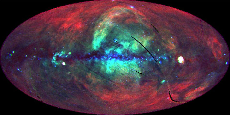
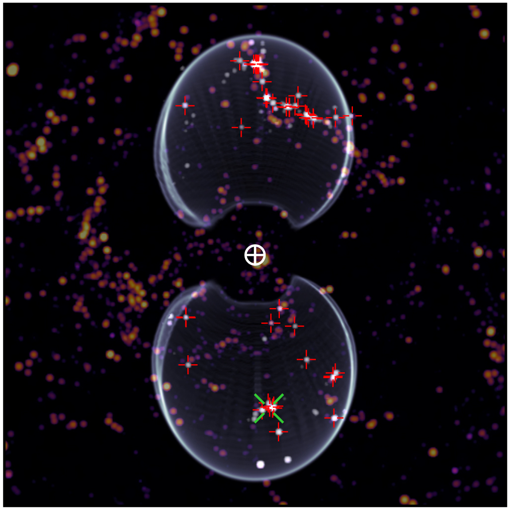
ROSAT image of the soft X-ray background throughout the universe. The different colors represent different energy bands: 0.25 keV (red), 0.75 keV (green), 1.5 keV (blue). [NASA/ROSAT Project]

Understanding this time period — in particular, determining what sources caused the reionization, and what the properties were of the gas strewn throughout the universe during this time — is necessary for us to be able to correctly interpret cosmological observations.

Conveniently, the universe has provided us with an interesting clue: the large-scale, diffuse X-ray background we observe all around us. What produced these X-rays, and what impact did this radiation have on the intergalactic medium long ago?

The First Binaries

A team of scientists led by Hao Xu (UC San Diego) has suggested that the very first generation of stars might be an important contributor to these X-rays.

This hypothetical first generation, Population III stars, are thought to have formed before and during reionization from large clouds of gas containing virtually no metals. Studies suggest that a large fraction of Pop III stars formed in binaries — and when those stars ended their lives as black holes, ensuing accretion from their companions could produce X-ray radiation.

The evolution with redshift the authors find for the mean X-ray background intensities. Each curve represents a different observed X-ray energy (and the total X-ray background is given by the sum of the curves). The two panels show results from two different calculation methods. [Xu et al. 2016]

The evolution with redshift of the mean X-ray background intensities. Each curve represents a different observed X-ray energy (and the total X-ray background is given by the sum of the curves). The two panels show results from two different calculation methods. [Xu et al. 2016]

Xu and collaborators have now attempted to model to the impact of this X-ray production from Pop III binaries on the intergalactic medium and determine how much it could have contributed to reionization and the diffuse X-ray background we observe today.

Generating a Background

The authors estimated the X-ray luminosities from Pop III binaries using the results of a series of galaxy-formation simulations, beginning at a redshift of z ~ 25 and evolving up to z = 7.6. They then used these luminosities to calculate the resulting X-ray background.

Xu and collaborators find that Pop III binaries can produce significant X-ray radiation throughout the period of reionization, and this radiation builds up gradually into an X-ray background. The team shows that X-rays from Pop III binaries might actually dominate more commonly assumed sources of the X-ray background at high redshifts (such as active galactic nuclei), and this radiation is strong enough to heat the intergalactic medium to 1000K and ionize a few percent of the neutral hydrogen.

If Pop III binaries are indeed this large of a contributor to the X-ray background and to the local and global heating of the intergalactic medium, then it’s important that we follow up with more detailed modeling to understand what this means for our interpretation of cosmological observations.

Citation

Hao Xu et al 2016 ApJL 832 L5. doi:10.3847/2041-8205/832/1/L5

SuperTIGER launch

cosmic-ray impact

Illustration of cosmic-ray nuclei impacting Earth’s atmosphere and decaying into lighter particles. [ESA]

The SuperTIGER (Trans-Iron Galactic Element Recorder) experiment flew over Antarctica for 55 days, collecting millions of galactic cosmic rays. What can it tell us about the origins of these high-energy particles?

High-Energy Impacts

Galactic cosmic rays are immensely high-energy protons and atomic nuclei that impact our atmosphere, originating from outside of our solar system. Where do they come from, and how are they accelerated? These are both open topics of research.

One of the leading theories is that cosmic-ray source material is primarily a mixture of material that has been ejected from massive stars — either from supernovae or in stellar wind outflows — and normal interstellar medium (ISM). This material is then accelerated to cosmic-ray energies by supernova shocks.

charge histogram

Number of nuclei of each element detected by SuperTIGER. Note the change of scale between the two plots (click for a closer look)! [Murphy et al. 2016]

How can we test this model? An important step is understanding the composition of galactic cosmic rays: what elemental nuclei are they made up of? If abundances are similar to solar-system abundances, then the material is likely mostly ISM. If the abundances of rarer heavy elements are high, however, then the material is more likely to have come from massive stars in star-forming regions.

Balloon-Borne Detections

Enter SuperTIGER, an experiment designed to collect cosmic rays and measure the abundances of the rare heavy elements — those with atomic number between iron (Z=26) and zirconium (Z=40).

SuperTIGER path

The path that SuperTIGER took over Antarctica during its flight, with a different color denoting each circuit around the pole. Note where it got stuck in an eddy over the Transarctic Mountains at the end of its second circuit! [Columbia Scientific Balloon Facility]

To gather galactic cosmic rays, the detector must be above the Earth’s atmosphere; interactions with the atmosphere cause these particles to decay into lower-energy secondary particles upon impact. In addition, the detector must operate for a long time in order to make meaningful abundance measurements: millions of cosmic-ray detections can result in just a few hundreds of detections of heavy-element nuclei.

The SuperTIGER team solved these problems by flying their instrument on a high-altitude scientific balloon at 127,000 feet. The project launched in Antarctica, taking advantage of the wind patterns circulating around the pole to maximize the flight time. In the end, SuperTIGER flew for 55 days, shattering the record for longest flight of a heavy-lift scientific balloon (which was previously 42 days). During this time, the experiment detected a whopping 50 million cosmic rays.

Pinning Down Abundances

elemental abundances

Measured elemental abundances for galactic cosmic rays, from SuperTIGER (orange) and other experiments. [Murphy et al. 2016]

Now, in a publication led by Ryan Murphy (Washington University in St. Louis), the team has detailed the results of SuperTIGER’s observations. Their measurements represent the tightest constraints on the abundances of galactic cosmic ray nuclei made in this charge and energy range, and the abundances are consistent with a model in which source material consists of a mixture of 19% material from massive stars and 81% normal ISM.

These results support the idea that a significant fraction of cosmic-ray material originates in associations of young, massive stars, and that the remainder is made up of solar-system-abundance ISM that’s injected and accelerated — possibly by supernova shocks — into cosmic rays.

Citation

R. P. Murphy et al 2016 ApJ 831 148. doi:10.3847/0004-637X/831/2/148

hot Jupiter

We know that the large masses of stars govern the orbits of the planets that circle them — but a large, close-in planet can also influence the rotation of its host star. A recently discovered, unusual hot Jupiter may be causing its star to spin faster than it should.

Exotic Planets

Hot Jupiters are gas giants of roughly Jupiter’s size that orbit close in to their host stars. Though these planets are easy to detect — their large sizes and frequent transits mean surveys have a good chance of catching them — we haven’t found many of them, suggesting that planetary systems containing hot Jupiters are fairly unusual.

HATS-18 light curve

The period-folded light curve of HATS-18, revealing the transit of the hot Jupiter HATS-18b. The period is P=0.8378 days. [Penev et al. 2016]

Studying this exotic population of planets, however, can help us to better understand how gas giants form and evolve in planetary systems. New observations of hot Jupiters may also reveal how stars and close-in planets interact through radiation, gravity, and magnetic fields.

The recent discovery of a transiting hot Jupiter a little over 2000 light-years away therefore presents an exciting opportunity!

A Speeding Giant

The discovery of HATS-18b, a planet of roughly 2 times Jupiter’s mass and 1.3 times its radius, was announced in a study led by Kaloyan Penev (Princeton University). The planet was discovered using the HATSouth transit survey network, which includes instruments in Chile, Namibia, and Australia, and follow-up photometry and spectroscopy was conducted at a variety of ground-based observatories.

HATS-18b’s properties are particularly unusual: this hot Jupiter is zipping around its host star — which is very similar to the Sun — at the incredible pace of one orbit every 0.84 days. HATS-18b’s orbit is more than 20 times closer to its host star than Mercury’s is to the Sun, bringing it so close it nearly grazes the star’s surface!

orbit vs. stellar rotation period

Size of the planetary orbit relative to the stellar radius as a function of the stellar rotation period, for transiting planets with orbital periods shorter than 2 days and masses greater than 0.1 Jupiter masses. HATS-18b is denoted by the red star. [Penev et al. 2016]

Tidal Interactions

What happens when a massive planet orbits this close to its star? Tidal interactions between the star and the planet cause tidal dissipation in the star, resulting in decay of the planet’s orbit. But there may be an additional effect of this interaction in the case of HATS-18b, the authors claim: the planet may be transferring some of its angular momentum to the star.

As stars age, they should gradually spin slower as they lose angular momentum via stellar winds. But Penev and collaborators note that this exoplanet’s host star, HATS-18, spins roughly three times as fast as its inferred age suggests it should. The authors conclude that the angular momentum lost by the planet as its orbit shrinks is deposited in the star, causing the star to spin up.

HATS-18 is an excellent laboratory for studying how very short-period planets interact with their stars — in fact, Penev and collaborators have already used their observations of the system to constrain models of tidal dissipation from Sun-like stars. Additional observations of HATS-18 and other short-period systems should allow us to further test models of how planetary systems form and evolve.

Citation

K. Penev et al 2016 AJ 152 127. doi:10.3847/0004-6256/152/5/127

LISA

Artist’s impression of the European Space Agency’s Laser Interferometer Space Antenna, currently planned for a 2034 launch. [NASA]

How are black-hole binaries built? Observations of gravitational waves from these systems — made using the European Space Agency’s upcoming mission, the Laser Interferometer Space Antenna (LISA) — may be able to reveal their origins.

Formation Channels

There are two primary places where stellar-mass black-hole binaries are thought to form:

  1. In isolation in the galactic field, as the components of a stellar binary independently evolve into black holes but remain bound to each other.
  2. In dense stellar environments like globular clusters, where the high density of already-formed black holes can cause a pair to dynamically interact and form a binary before being ejected from the cluster.

Can we differentiate between these origins based on future detections of gravitational waves from black-hole binaries? A team of scientists led by Katelyn Breivik (CIERA, Northwestern University) thinks that we can!

GW spectrum

The gravitational-wave spectrum and how we detect it (click for a closer look!). While ground-based interferometers like LIGO detect black-hole binaries in the final moments before merger, LISA’s lower frequency band will allow it to detect binaries earlier in their inspiral. [NASA Goddard SFC]

Differentiation by Eccentricity

Breivik and collaborators believe that the key clue is the binary’s eccentricity. Gravitational-wave emission will eventually circularize all black-hole binaries during their inspiral. But in the first formation scenario, binary evolution processes like tidal circularization and mass transfer will reduce the binary’s eccentricity early on — whereas in the second scenario, the binaries that form in globular clusters may retain eccentricity in their orbits long enough that we can detect it.

Ground-based interferometers won’t be up to this task; by the time the binary orbits shrink enough to evolve into the LIGO frequency band, the orbits won’t have measurable eccentricity anymore. But the upcoming space-based LISA mission, which will operate in a lower frequency band, might be able to pick up this signature.

To determine if LISA can pull it off, Breivik and collaborators simulate two populations of binary black holes: one evolved in isolation in galactic fields, and the other formed dynamically in globular clusters and then ejected. The authors then explore the evolution of these populations’ masses and eccentricities as their orbits narrow into the LISA-detectable frequency band.

Eccentricity evolution

Eccentricity evolution tracks as a function of gravitational-wave frequency for black-hole binaries formed in dynamical scenarios (black) and in isolation (blue for those with a common-envelope episode, green for those without). Eccentricities above 10-2 are measurable for all binaries; those above 10-3 are measurable for 90%. LISA’s frequency band is shown in grey. [Breivik et al. 2016]

Separating Populations

Breivik and collaborators find that LISA will be able to make several important distinctions. First, if LISA detects binary black holes with eccentricities of e > 0.01 at frequencies above 10-2 Hz, we can be fairly certain that these originated from dynamical processes in dense stellar environments.

For binary black holes detected with eccentricities of e > 0.01 at lower frequencies, they could either have formed in dense stellar environments or they could have formed in isolation. Based on this study’s results, however, those with measurable eccentricities that formed in isolation most likely originated from a common-envelope formation. Measuring eccentricities of such systems in the future could provide constraints on the physics of how this formation mechanism works.

Though the field of gravitational-wave astronomy is only just beginning, its future is promising! Theoretical studies like this one will help us to extract a greater understanding from the observations we can expect down the road.

Bonus

Check out this beautiful simulation from Northwestern Visualization and Carl Rodriguez (a co-author on the above study) that shows what the formation of a binary black hole in a globular cluster might look like!

Citation

Katelyn Breivik et al 2016 ApJL 830 L18. doi:10.3847/2041-8205/830/1/L18

solar cycle

Solar-like stars exhibit magnetic cycles; our Sun, for instance, displays an 11-year period in its activity, manifesting as cyclic changes in radiation levels, the number of sunspots and flares, and ejection of solar material. Over the span of two activity cycles, the Sun’s magnetic field flips polarity and then returns to its original state.

TRAPPIST-1

An artist’s illustration comparing the Sun to TRAPPIST-1, an ultracool dwarf star known to host several planets. [ESO]

But what about the magnetic behavior of objects near the cooler end of the stellar main sequence — do they exhibit similar activity cycles?

Effects of a Convecting Interior

Dwarf stars have made headlines in recent years due to their potential to harbor exoplanets. Because these cooler stars have lower flux levels compared to the Sun, their habitable zones lie much closer to the stars. The magnetic behavior of these stars is therefore important to understand: could ultracool dwarfs exhibit solar-like activity cycles that would affect planets with close orbits?

stellar interiors

The differences in internal structure between different mass stars. Ultracool dwarfs have fully convective interiors. [www.sun.org]

There’s a major difference between ultracool dwarfs (stars of spectral type higher than M7 and brown dwarfs) and Sun-like stars: their internal structures. Sun-like stars have a convective envelope that surrounds a radiative core. The interiors of cool, low-mass objects, on the other hand, are fully convective.

Based on theoretical studies of how magnetism is generated in stars, it’s thought that the fully convective interiors of ultracool dwarfs can’t support large-scale magnetic field formation. This should prevent these stars from exhibiting activity cycles like the Sun. But recent radio observations of dwarf stars have led scientist Matthew Route (ITaP Research Computing, Purdue University) to question these models.

A Reversing Field?

During observations of the brown dwarf star J1047+21 in 2010–2011, radio flares were detected with emission primarily polarized in a single direction. The dwarf’s flares in late 2013, however, all showed polarization in the opposite direction. Could this be an indication that J1047+21 has a stable, global dipolar field that flipped polarity in between the two sets of observations? If so, this could mean that the star has a magnetic cycle similar to the Sun’s.

stellar types

Artist’s impression showing the relative sizes and colors of the Sun, a red dwarf (M-dwarf), a hotter brown dwarf (L-dwarf), a cool brown dwarf (T-dwarf) similar to J1047+21, and the planet Jupiter [Credit: NASA/IPAC/R. Hurt (SSC)]

Inspired by this possibility, Route conducted an investigation of the long-term magnetic behavior of all known radio-flaring ultracool dwarfs, a list of 14 stars. Using polarized radio emission measurements, he found that many of his targets exhibited similar polarity flips, which he argues is evidence that these dwarfs are undergoing magnetic field reversals on roughly decade-long timescales, analogous to those reversals that occur in the Sun.

If this is indeed true, then we need to examine our models of how magnetic fields are generated in stars: the interface between the radiative and convective layers may not be necessary to produce large-scale magnetic fields. Understanding this process is certainly an important step in interpreting the potential habitability of planets around ultracool dwarfs.

Citation

Matthew Route 2016 ApJL 830 L27. doi:10.3847/2041-8205/830/2/L27

pulsar white dwarf binary

Astronomers have discovered a binary system consisting of a low-mass white dwarf and a millisecond pulsar — but its eccentric orbit defies all expectations of how such binaries form.

ms pulsar binaries

Observed orbital periods and binary eccentricities for binary millisecond pulsars. PSR J2234+0511 is the furthest right of the green stars that mark the five known eccentric systems. [Antoniadis et al. 2016]

Unusual Eccentricity

It would take a low-mass (<0.4 solar masses) white dwarf over 100 billion years to form from the evolution of a single star. Since this is longer than the age of the universe, we believe that these lightweights are instead products of binary-star evolution — and indeed, we observe many of these stars to still be in binary systems.

But the binary evolution that can create a low-mass white dwarf includes a period of mass transfer, in which efficient tidal dissipation damps the system’s orbital eccentricity. Because of this, we would expect all systems containing low-mass white dwarfs to have circular orbits.

In the past, our observations of low-mass white dwarf–millisecond pulsar binaries have all been consistent with this expectation. But a new detection has thrown a wrench in the works: the unambiguous identification of a low-mass white dwarf that’s in an eccentric (e=0.13) orbit with the millisecond pulsar PSR J2234+0511. How could this system have formed?

Eliminating Formation Models

Led by John Antoniadis (Dunlap Institute at University of Toronto), a team of scientists has used newly obtained optical photometry (from the Sloan Digital Sky Survey) and spectroscopy (from the Very Large Telescope in Chile) of the white dwarf to confirm the identification of this system.

Antoniadis and collaborators then use measurements of the bodies’ masses (0.28 and 1.4 solar masses for the white dwarf and pulsar, respectively) and velocities, and constraints on the white dwarf’s temperature, radius and surface gravity, to address three proposed models for the formation of this system.

  1. pulsar motion

    The 3D motion of the pulsar (black solid lines; current position marked with diamond) in our galaxy over the past 1.5 Gyr. This motion is typical for low-mass X-ray binary descendants, favoring a binary-evolution model over a 3-body-interaction model. [Antoniadis et al. 2016]

    In the first model, the eccentric binary was created via a dynamic three-body formation channel. This possibility is deemed unlikely, as the white-dwarf properties and all the kinematic properties of the system point to normal binary evolution.
  2. In the second model, the binary system gains its high eccentricity after mass transfer ends, when the pulsar progenitor experiences a spontaneous phase transition. The authors explore two options for this: one in which the neutron star implodes into a strange-quark star, and the other in which an over-massive white dwarf suffers a delayed collapse into a neutron star. Both cases are deemed unlikely, because the mass inferred for the pulsar progenitor is not consistent with either model.
  3. In the third model, the system forms a circumbinary disk fueled by material escaping the proto-white dwarf. After mass transfer has ended, interactions between the binary and its disk gradually increase the eccentricity of the system, pumping it up to what we observe today. All of the properties of the system measured by Antoniadis and collaborators are thus far consistent with this model.

Further observations of this system and systems like it (several others have been detected, though not yet confirmed) will help determine whether binary evolution — combined with interactions with a disk — can indeed explain the formation of this unexpectedly eccentric system.

Citation

John Antoniadis et al 2016 ApJ 830 36. doi:10.3847/0004-637X/830/1/36

Vesta

How can we tell what an asteroid is made of? Until now, we’ve relied on remote spectral observations, though NASA’s recently launched OSIRIS-REx mission may soon change this by landing on an asteroid and returning with a sample.

But what if we could learn more about the asteroids near Earth without needing to land on each one? It turns out that we can — by flying through their dust.

Aerogel

The aerogel dust collector of the Stardust mission. [NASA/JPL/Caltech]

Ejected Clues

When an airless body is impacted by the meteoroids prevalent throughout our solar system, ejecta from the body are flung into the space around it. In the case of small objects like asteroids, their gravitational pull is so weak that most of the ejected material escapes, forming a surrounding cloud of dust.

By flying a spacecraft through this cloud, we could perform chemical analysis of the dust, thereby determining the asteroid’s composition. We could even capture some of the dust during a flyby (for example, by using an aerogel collector like in the Stardust mission) and bring it back home to analyze.

So what’s the best place to fly a dust-analyzing or -collecting spacecraft? To answer this, we need to know what the typical distribution of dust is around a near-Earth asteroid (NEA) — a problem that scientists Jamey Szalay (Southwest Research Institute) and Mihály Horányi (University of Colorado Boulder) address in a recent study.

Dust distribution

The colors show the density distribution for dust grains larger than 0.3 µm around a body with a 10-km radius. The distribution is asymmetric, with higher densities on the apex side, shown here in the +y direction. [Szalay & Horányi 2016]

Moon as a Laboratory

To determine typical dust distributions around NEAs, Szalay and Horányi first look at the distribution of dust around our own Moon, caused by the same barrage of meteorites we’d expect to impact NEAs. The Moon’s dust cloud was measured in situ in 2013 and 2014 by the Lunar Dust Experiment (LDEX) on board the Lunar Atmosphere and Dust Environment Explorer mission.

From LDEX’s measurements of the dust distribution around the Moon, Szalay and Horányi next calculate how this distribution would change for different grain sizes if the body were instead much smaller — i.e., a 10-km asteroid instead of the 1700-km Moon.

Optimizing the Geometry for an Encounter

The authors find that the dust ejected from asteroids is distributed in an asymmetric shape around the body, with higher dust densities on the side of the asteroid facing its direction of travel. This is because meteoroid impacts aren’t isotropic: meteoroid showers tend to be directional, and a majority of meteoroids impact the asteroid from this “apex” side.

flyby trajectories

Total number of impacts per square meter and predicted dust density for a family of potential trajectories for spacecraft flybys of a 10-km asteroid. [Szalay & Horányi 2016]

Szalay and Horányi therefore conclude that dust-analyzing missions would collect many times more dust impacts by transiting the apex side of the body. The authors evaluate a family of trajectories for a transiting spacecraft to determine the density of dust that the spacecraft will encounter and the impact rates expected from the dust particles.

This information can help optimize the encounter geometry of a future mission to maximize the science return while minimizing the hazard due to dust impacts.

Citation

Jamey R. Szalay and Mihály Horányi 2016 ApJL 830 L29. doi:10.3847/2041-8205/830/2/L29

superluminous supernova

What causes the tremendous explosions of superluminous supernovae? New observations reveal the geometry of one such explosion, SN 2015bn, providing clues as to its source.

A New Class of Explosions

supernova

Image of a type Ia supernova in the galaxy NGC 4526. [NASA/ESA]

Supernovae are powerful explosions that can briefly outshine the galaxies that host them. There are several different classifications of supernovae, each with a different physical source — such as thermonuclear instability in a white dwarf, caused by accretion of too much mass, or the exhaustion of fuel in the core of a massive star, leading to the core’s collapse and expulsion of its outer layers.

In recent years, however, we’ve detected another type of supernovae, referred to as “superluminous supernovae”. These particularly energetic explosions last longer — months instead of weeks — and are brighter at their peaks than normal supernovae by factors of tens to hundreds.

The physical cause of these unusual explosions is still a topic of debate. Recently, however, a team of scientists led by Cosimo Inserra (Queens University Belfast) has obtained new observations of a superluminous supernova that might help address this question.

polarization

The flux and the polarization level (black lines) along the dominant axis of SN 2015bn, 24 days before peak flux (left) and 28 days after peak flux (right). Blue lines show the author’s best-fitting model. [Inserra et al. 2016]

Probing Geometry

Inserra and collaborators obtained two sets of observations of SN 2015bn — one roughly a month before and one a month after the superluminous supernova’s peak brightness — using a spectrograph on the Very Large Telescope in Chile. These observations mark the first spectropolarimetric data for a superluminous supernova.

Spectropolarimetry is the practice of obtaining information about the polarization of radiation from an object’s spectrum. Polarization carries information about broken spatial symmetries in the object: only if the object is perfectly symmetric can it emit an unpolarized spectrum. Otherwise, the polarization of an object’s spectrum reveals information about its geometry.

Modeling Ejecta

SN 2015bn model

The authors’ best model of the geometry of SN 2015bn 24 days before (top) and 28 days after (bottom) peak flux. The model consists of two ellipsoidal layers of ejecta material. [Inserra et al. 2016]

Based on their observations, Inserra and collaborators find that SN 2015bn is not spherically symmetric — but it does appear to be axisymmetric around a single dominant axis. They also find that the polarization level of the object changes both with wavelength and over time.

To explain these dependencies, the authors produce a simple toy model of SN 2015bn. In the best-fitting model, the supernova has a two-layered ellipsoidal or bipolar geometry. The inner region becomes more and more aspherical as time passes.

What does this model tell us about the physical cause of this superluminous supernova? Inserra and collaborators argue that the axisymmetric shape favors a core-collapse explosion. A central inner engine of a spinning magnetar (a highly magnetized neutron star) or black hole then remains at the center of this explosion, pumping energy into it and causing the increase of the inner asymmetry over time.

The authors caution that their models are very preliminary — but these observations should drive future, more detailed modeling, as well as further spectropolarimetric observations of future nearby superluminous supernovae. With luck, we will soon better understand what drives these unusual explosions.

Citation

C. Inserra et al 2016 ApJ 831 79. doi:10.3847/0004-637X/831/1/79

GW150914 location

Now that we’re able to detect gravitational waves, the next challenge is to spot electromagnetic signatures associated with gravitational-wave events. A team of scientists has proposed a new algorithm that might narrow the search.

electromagnetic counterparts

Artist’s illustrations of the stellar-merger model for short gamma-ray bursts. In the model, 1) two neutron stars inspiral, 2) they merge and produce a gamma-ray burst, 3) a small fraction of their mass is flung out and radiates as a kilonova, 4) a massive neutron star or black hole with a disk remains after the event. [NASA, ESA, and A. Feild (STScI)]

Light from Neutron-Star Mergers

Just over a year ago, LIGO detected its first gravitational-wave signal: GW150914, produced when two black holes merged. While we didn’t expect to see any sort of light-based signal from this merger, we could expect to see transient electromagnetic signatures in the case of a neutron star–black hole merger or a neutron star–neutron star merger — in the form of a kilonova or a short gamma-ray burst.

While we haven’t yet detected any mergers involving neutron stars, LIGO has the sensitivity to make these detections in the local universe, and we hope to start seeing them soon! Finding the electromagnetic companions to gravitational-wave signals would be the best way to probe the evolution history of the universe and learn what happens when evolved stars collide. So how do we hunt them down?

GW150914 LIGO localization

2D localization maps for LIGO’s detection of GW150914 (black contours), as well as the footprints of follow-up observations (red for radio, green for optical/IR, blue for X-ray). [Abbott et al. 2016]

Pinpointing a Volume

The two LIGO detectors can already provide rough 2D localization of where the gravitational-wave signal came from, but the region predicted for GW150914 still covered 600 square degrees, which is a pretty hefty patch of sky! In light of this, the simplest follow-up strategy of tiling large survey observations of the entire predicted region is somewhat impractical and time-consuming. Could we possibly take a more targeted approach?

The key, say a team of scientists led by Leo Singer (NASA Goddard SFC), is in using 3D estimates of the source location, rather than 2D sky maps: we need to produce distance estimates for the gravitational-wave source as well. Singer and collaborators have developed an algorithm that, from a gravitational-wave signal, can produce a fast full-volume estimate of the probability distribution for its source’s location.

Predicted volume

Volume rendering of the 90% credible region for a simulated gravitational-wave event, superimposed over a galaxy map for the region. Green crosshairs represent the true location of the source; the most massive galaxies inside the credible region are highlighted. Searching only these galaxies could significantly reduce the observing time needed to detect an electromagnetic counterpart. [Singer et al. 2016]

We can then easily cross-reference the volume predicted to contain the source against a galaxy catalog to identify the most probable host galaxies for the signal. This approach allows us to target specific galaxies for rapid observations with follow-up campaigns in the search for a counterpart.

Targeted Efficiency

Singer and collaborators’ approach would make searching for electromagnetic counterparts to gravitational-wave events a much more efficient process. One particular advantage would be in reducing the number of false positives: for a typical wide-field follow-up campaign searching ~100 square degrees, hundreds of contaminating supernovae would be in the field. Targeting only 10’ x 10’ patches around 100 nearby galaxies, however, reduces the background to fewer than 10 contaminating supernovae.

An additional benefit is that this targeted strategy opens the door of gravitational-wave follow-up to many small-field-of-view, large-aperture telescopes, instead of limiting the task to broad synoptic surveys. This permits the involvement of many more campaigns in the hunt for the important electromagnetic counterparts to gravitational waves.

Note: Want to check out the team’s data? It’s publicly available here!

Citation

Leo P. Singer et al 2016 ApJL 829 L15. doi:10.3847/2041-8205/829/1/L15

galactic nucleus

The recent discovery of old and variable RR Lyrae stars in the very center of our galaxy may answer the long-standing question of how the Milky Way’s nucleus formed.

Models for a Dense Nucleus

Milky Way

Face-on illustration of the Milky Way’s structure. The galactic nucleus makes up a very small component of the galaxy; it extends roughly 400 light-years from the Milky Way’s center. Compare this to the 100,000 light-year total diameter of the galaxy! [NASA/Robert Hurt]

The nuclei of galaxies are extreme regions that typically host a supermassive black hole and extremely high stellar densities. The Milky Way’s nuclear bulge is no exception, consisting observationally of two components: the extremely dense and compact nuclear star cluster, which dominates the inner 100 light-years, and the nuclear stellar bulge, a component which extends out to about 400 light-years.

How galactic nuclei like the Milky Way’s formed remains an open question today. Two possible scenarios have been proposed:

  1. Fast gas accretion onto the central region caused rapid star formation, leading to the high stellar densities in the nucleus.
  2. Globular clusters sank to the center of the galaxy via dynamical friction, where they merged and formed the high-density nuclear bulge with the nuclear star cluster at its center.

How can we test the second model? A huge point of support would be the discovery of stars in the nuclear bulge that are characteristically found in old Milky Way globular clusters. No surveys, however, have been able to probe deep enough to find such old, faint stars amidst the bright stars that have formed more recently — until now.

Tell-Tale Stars

Led by Dante Minniti (Millennium Institute of Astrophysics and Andres Bello National University, Chile; Vatican Observatory), a team of scientists has now presented data from the VISTA Variables in the Via Lactea (VVV) ESO public survey. VVV’s deep photometry in the near-infrared allowed Minniti and collaborators to discover a dozen faint RR Lyrae stars within ~275 light-years of the galactic center.

RR Lyrae light curves

Characteristic saw-tooth light curves for several of the old RR Lyrae stars discovered in the galactic nuclear bulge. [Minniti et al. 2016]

RR Lyrae stars are variable stars that are old and metal-poor, and are most commonly found in globular clusters. Their periodic pulsations mean that they can be used as standard candles, allowing for a precise measurement of their location in the nuclear bulge.

The discovery of these stars provides the first direct observational evidence that the galactic nuclear stellar bulge contains ancient stars, indicating that the galactic nucleus formed long ago (at least 10 billion years ago, if not more). The distribution of the RR Lyrae stars throughout the central region of our galactic nucleus supports the scenario in which these stars are the remains of primordial globular clusters that merged to form the nuclear bulge of the Milky Way.

If this scenario is correct, it would mean that the nuclear bulge is the most massive and oldest surviving star cluster of our galaxy! We hope to soon learn more about this population of old stars in the Milky Way’s nucleus, as an extended VVV survey is planned for the next three years.

Citation

Dante Minniti et al 2016 ApJ 830 L14. doi:10.3847/2041-8205/830/1/L14

1 95 96 97 98 99 113