
Can Computers Identify Holes in the Sun?
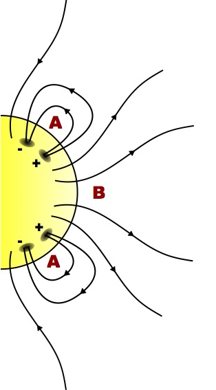
Coronal holes form where magnetic field lines open into space (B) instead of looping back to the solar surface (A). [Sebman81]
Tracking the Dark
The Sun’s outer atmosphere — its corona — is far from uniform. Both across the Sun’s face and over time, the corona varies in its density and corresponding appearance, looking brighter in some regions and forming large, dark coronal holes in others.
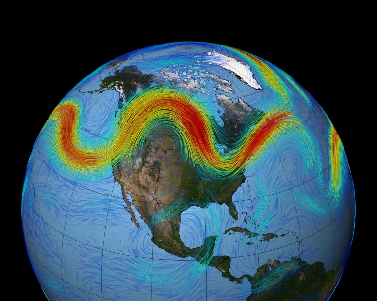
Coronal holes represent regions of low-density plasma containing magnetic field lines that open out into space rather than looping back down to the Sun’s surface. These areas of open field lines provide an excellent escape point for the solar wind, the high-energy particles that flow off of the Sun.
For this reason, identifying the locations, sizes, and timescales for formation and evolution of coronal holes is critical for predicting solar wind behavior and forecasting space weather. In addition, tracking coronal holes over solar cycles can shed light on how magnetic fields drive solar activity and may even help us to better predict upcoming solar activity.
A Full-Surface View
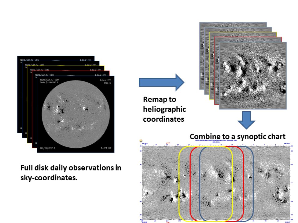
The process of making a synoptic map from daily solar disk images. Click to enlarge. [NSO]
To get a comprehensive view of the entire solar surface, we transform these individual disk images into a shared coordinate system, and then we stack and combine the daily images within each rotation period, creating what’s known as a synoptic map for each rotation.
If we can then identify the coronal holes in a uniform way within each of these synoptic maps, we’ll have a useful data set for studying how coronal holes vary across the Sun’s surface and over time! In a new publication, a team of scientists led by Egor Illarionov (Moscow State University, Russia) has found a way to do this that uses computers to do the heavy lifting.
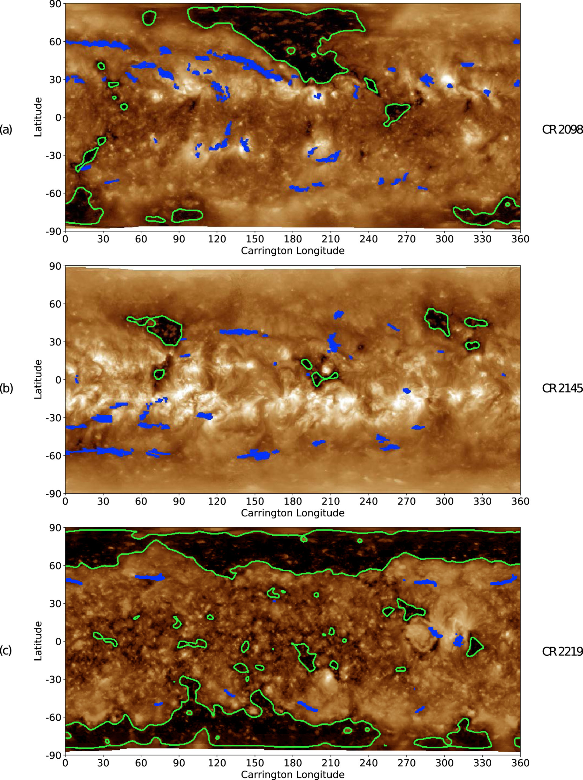
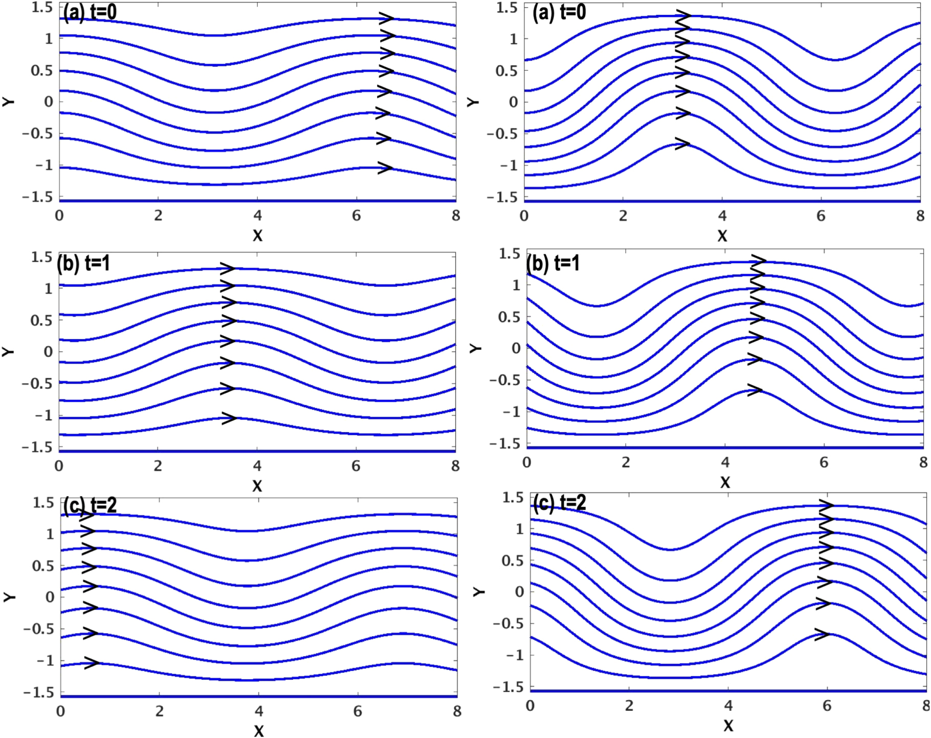
Overlaid synoptic maps and algorithm-identified coronal hole boundaries (green outlines) for three different solar rotation periods: two during solar minima (a and c) and one during a solar maximum (b). [Illarionov et al. 2020]
Training the Machine
Illarionov and collaborators use a training set of daily solar disk images to teach a convolutional neural network — a type of machine learning algorithm that’s especially good at analyzing images — how to identify coronal holes. The strength of a convolutional neural network is that it works equally well analyzing any image shape; the authors can therefore use this same algorithm, once trained, to accurately identify coronal holes in the synoptic solar maps.
Using this approach, Illarionov and collaborators construct a coronal hole catalog spanning 2010–2020. They conduct preliminary analysis of the evolution of coronal holes between solar minimum and solar maximum, and they compare these maps to maps of magnetic flux across the same times.
Looking to dive in, yourself? The authors make their code and the resulting coronal hole maps publicly available. With this dataset on hand, we can hope to soon learn more from these holes in the Sun.
Citation
“Machine-learning Approach to Identification of Coronal Holes in Solar Disk Images and Synoptic Maps,” Egor Illarionov et al 2020 ApJ 903 115. doi:10.3847/1538-4357/abb94d


