
Alignment of a Star and a Planet
The planets in our solar system all orbit in roughly the same direction as the Sun spins — but this isn’t true for all planetary systems! Recent measurements of the spin angle of a nearby, planet-hosting star provide new insight into how solar systems form.
The Birth of a Solar System
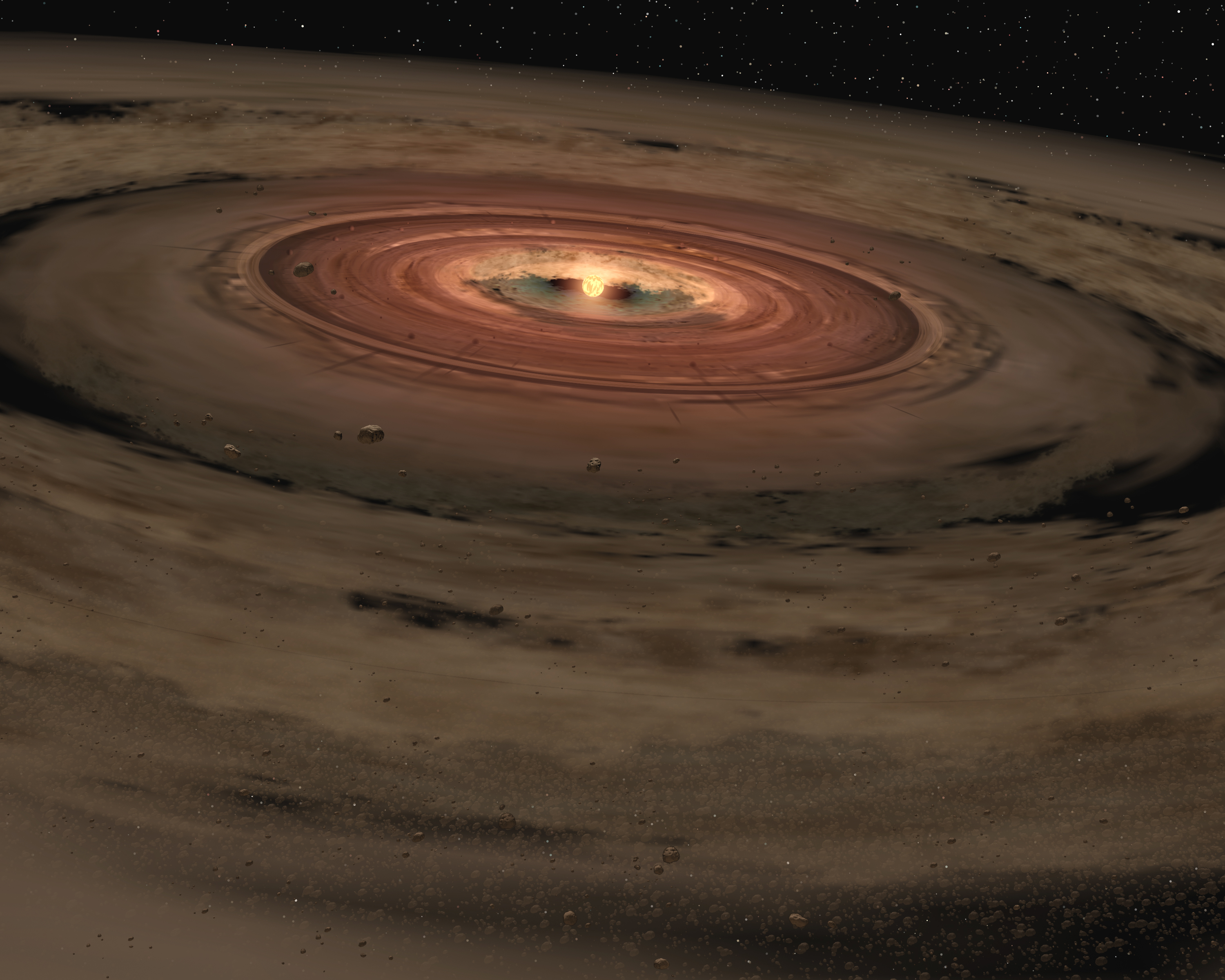
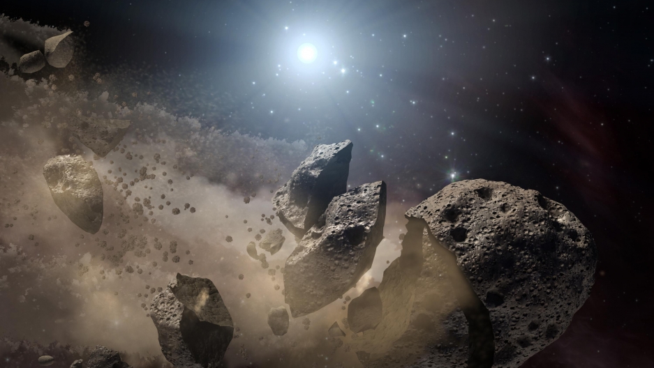
If planets form from the same rotating material that created their host star, why don’t all planets have orbits that are aligned with their stars’ spins? [NASA/JPL-Caltech]
In this picture, conservation of angular momentum suggests that the spin axis of a star should be aligned with the orbital angular momentum vectors of its planets — a state known as spin–orbit alignment.
This is true in our solar system: our planets’ orbits are aligned to within 7° of the Sun’s spin. But roughly a third of the planets we’ve measured in other systems have significant misalignments — ranging from slightly tilted orbits to orbits that are fully the opposite direction of their star’s spin.
Explaining Crooked Paths
There are two possible explanations for these misaligned orbits:
- A star’s spin and its planet-forming disk might be misaligned from the start — perhaps due to effects like turbulence or dynamical interactions in the star’s birth environment.
- Planet orbits and stellar spin start out aligned, but some planets get scattered or nudged onto misaligned orbits after they form.
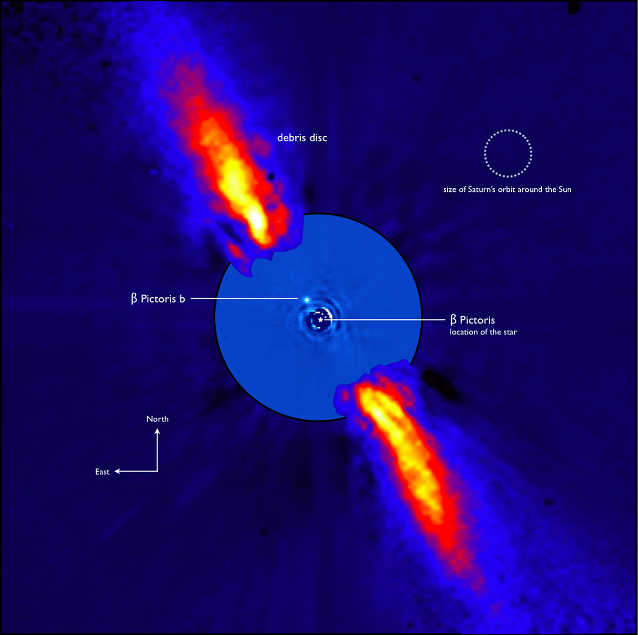
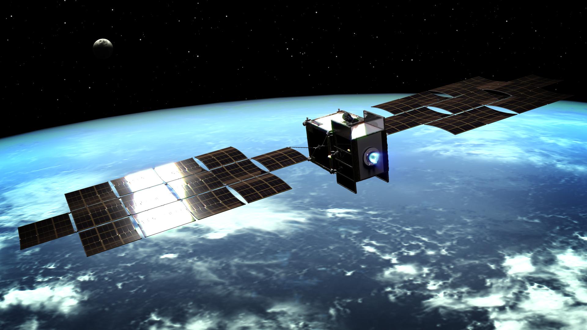
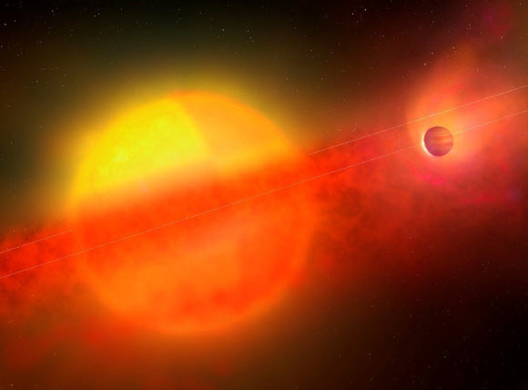
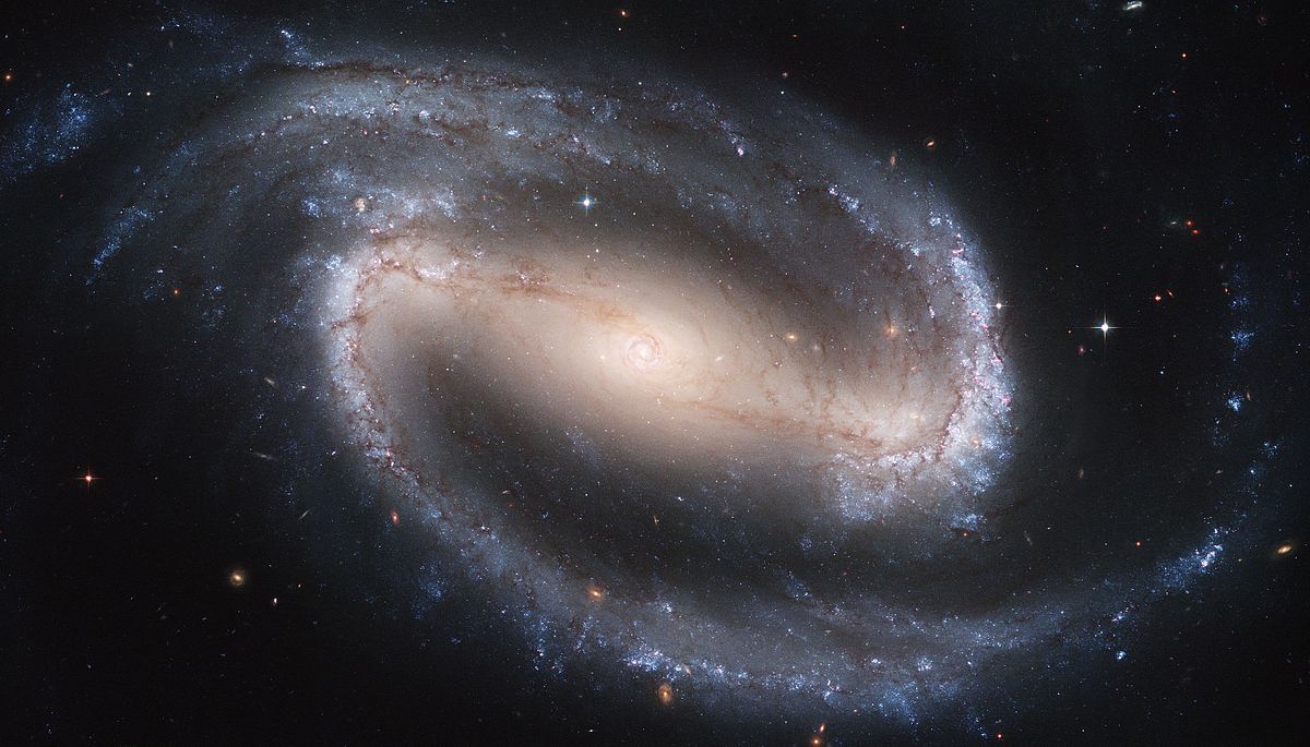
β Pictoris b is a directly imaged planet that orbits at ~10.6 AU from its host star, as seen at the center of this composite infrared image of the system. [ESO/A.-M. Lagrange et al.]
But to confirm that this explanation fits, we’d also need to show that the spin–orbit alignments of long–period planets — which are less likely to have been perturbed over their lifetimes — are typically aligned.
In a new study, a team of scientists led by Stefan Kraus (University of Exeter, UK) have now made the first measurement of the spin–orbit alignment of a directly imaged, wide-orbit exoplanet: β Pictoris b.
Confirmation from a Wide Orbiter
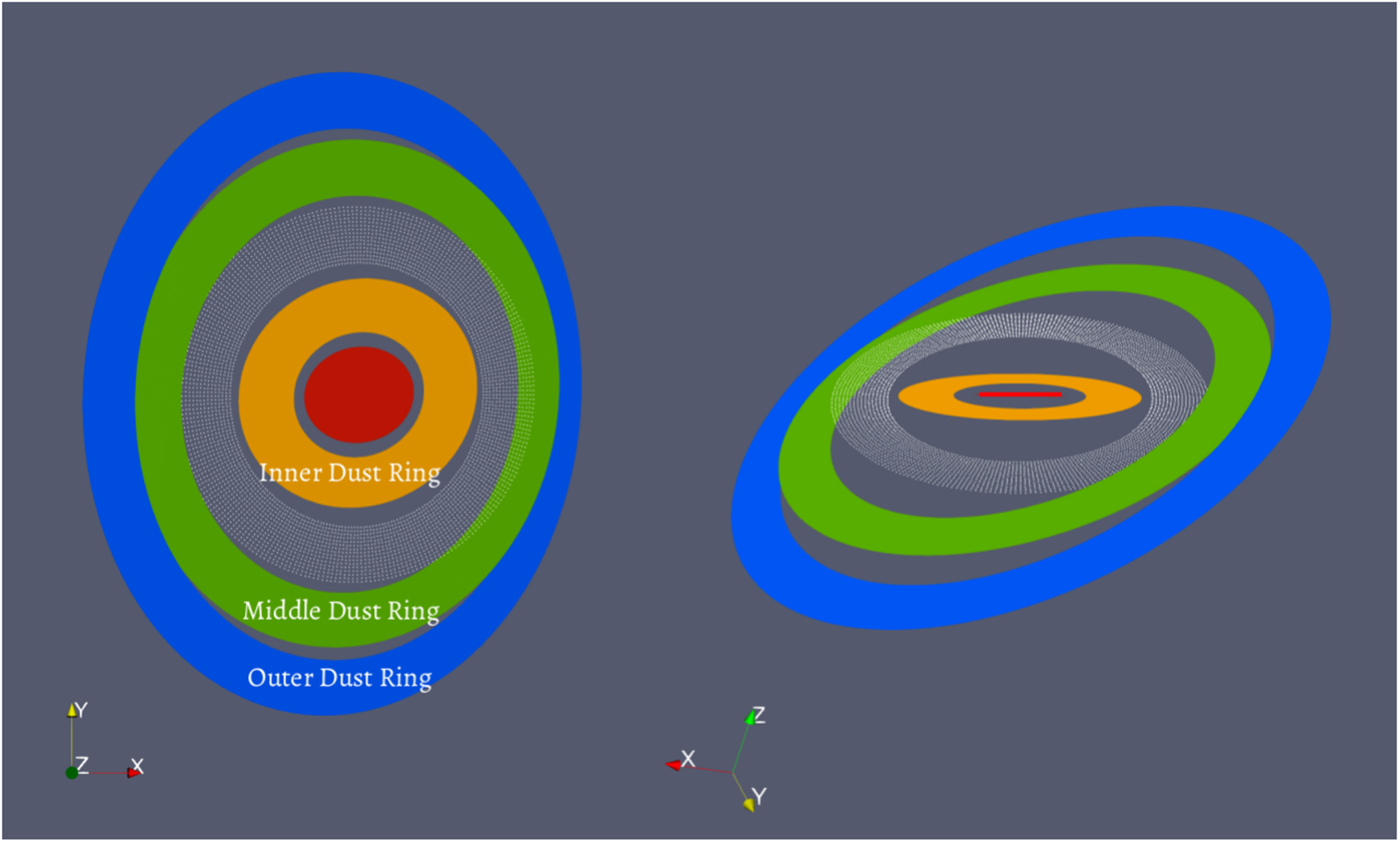
Located just ~60 light-years away, the recently formed star β Pictoris hosts a roughly 13-Jupiter-mass exoplanet — β Pictoris b — that orbits with a semimajor axis of 10.6 AU within a young debris disk that surrounds the star.
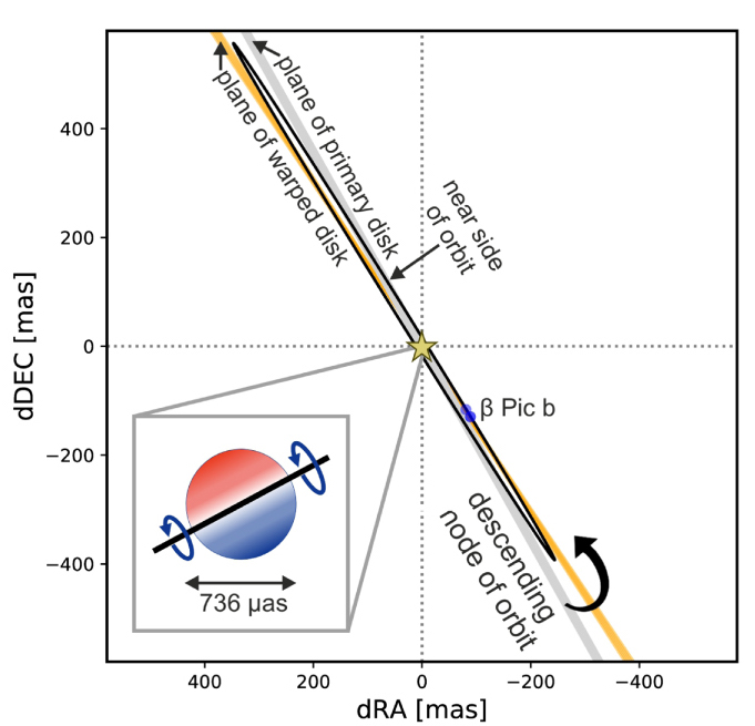
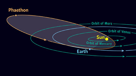
Schematic illustrating the components of the β Pictoris system. Click to enlarge. [Adapted from Kraus et al. 2020]
Kraus and collaborators’ results support the idea that solar systems initially form with aligned stellar spin and planet orbits; misalignments are introduced only later as planets migrate. Additional observations of wide-orbit planets will be needed to confirm this picture — but we can hope to gather more in the future using the techniques demonstrated in this study!
Citation
“Spin–Orbit Alignment of the β Pictoris Planetary System,” Stefan Kraus et al 2020 ApJL 897 L8. doi:10.3847/2041-8213/ab9d27


