A New Assessment of Supermassive Black Holes and Our Universe
Supermassive black holes influence many aspects of our universe’s formation and evolution — yet there’s still a lot we don’t know about them! A new census of these lurking sources is helping us to answer questions.
Hidden in Dust
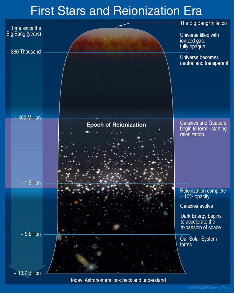
In the schematic timeline of the universe, the epoch of reionization is when the first galaxies and quasars began to form and evolve. Click to enlarge. [NASA]
To answer all these questions,we first need to form a complete census of the AGN in our universe. This prospect is challenging, however: though AGN radiate brightly across the electromagnetic spectrum, many of these mysterious sources lie obscured within dense shrouds of dust that prevent the majority of their radiation from escaping.
High Energy to the Rescue
Fortunately, however, extremely energetic X-ray radiation can escape even heavily obscured AGN. By compiling the observations from multiple space-based X-ray observatories — like NuSTAR, the Neil Gehrels Swift Observatory, and Chandra — a team of scientists has recently built a largely unbiased survey of the AGN throughout our universe, accounting for both unobscured sources and the many sources that are hidden by dust.
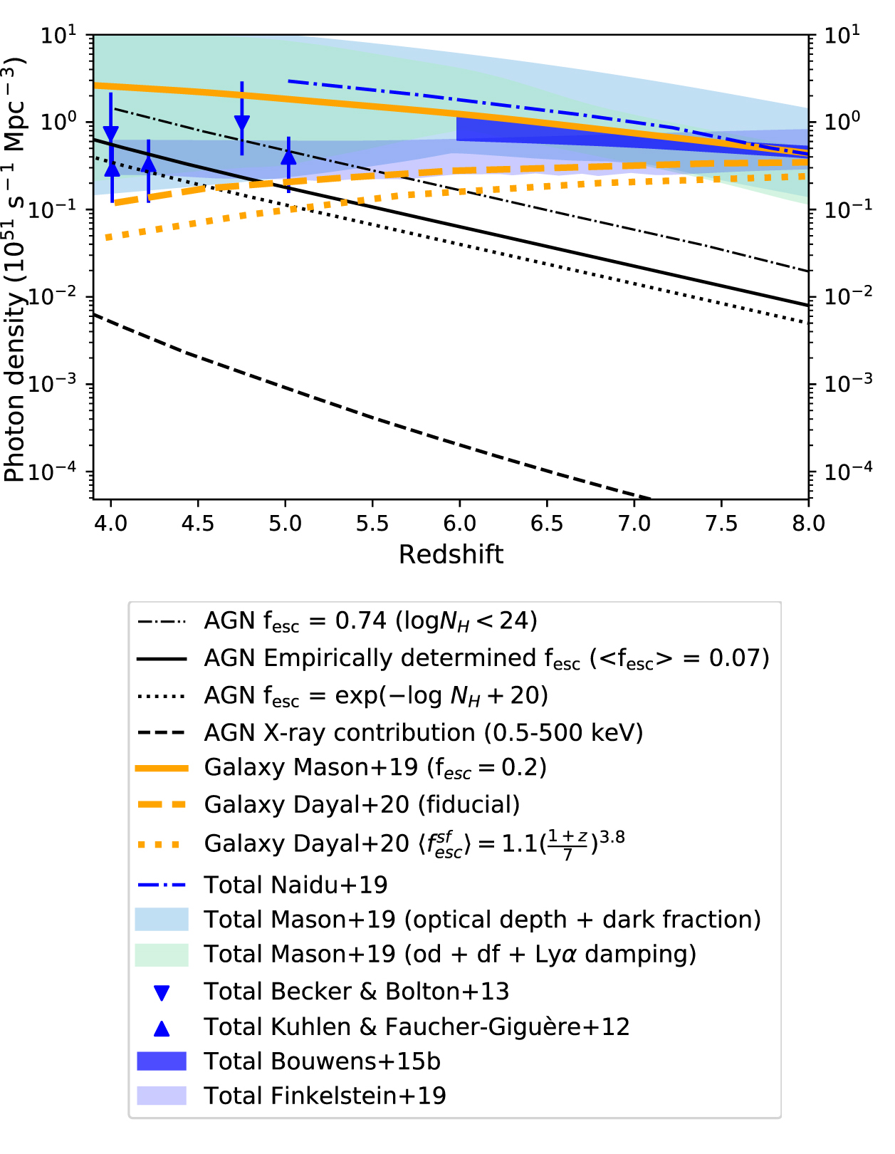
Ionizing photon densities for AGN (black lines) and galaxies (orange lines) for several different models. The authors’ work suggests that galaxies provide a substantially larger contribution toward reionization than AGN do, at redshifts above z = 6. [Adapted from Ananna et al. 2020]
Reionizing Our Universe
Ananna and collaborators estimate the total amount of ionizing radiation that’s emitted from all AGN in our universe as a function of redshift, applying observational constraints from both the light that we can see and estimates of the light we can’t see based on the inferred obscured AGN population.
The authors find that the total contribution of ionizing photons that escape from all AGNs is fairly small. The AGN contribution to the reionization of our universe — a process that occurred between a few hundred million and ~1 billion years after the Big Bang — is less than a quarter of the total ionizing photon density at redshifts larger than z > 6. This suggests that first-generation stars and galaxies contributed the vast majority of the radiation that drove reionization.
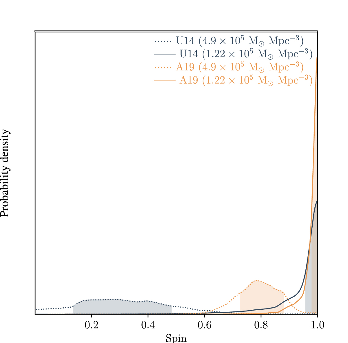
Authors’ probability distribution for the measurement of average black-hole spin among AGN, using several different models. High spins are significantly favored. [Adapted from Ananna et al. 2020]
Dizzy Black Holes
What can we learn about the black holes themselves? Ananna and collaborators use their census to compare the total light emitted from AGNs to the amount of mass they’ve accreted over time. This measure of accretion efficiency can then tell us how fast the supermassive black holes are likely spinning.
Ananna and collaborators find a high likely accretion efficiency — which indicates that, on average, growing supermassive black holes are spinning quite rapidly. If confirmed, this may mean that supermassive black hole growth is dominated by accretion of material (which produces fast-spinning black holes) rather than by mergers (which produce a low average spin since the black holes become randomly oriented).
We still have much to learn about supermassive black holes and their influence on the universe, but this recent study provides a clear step in the right direction.
Citation
“Accretion History of AGNs. III. Radiative Efficiency and AGN Contribution to Reionization,” Tonima Tasnim Ananna et al 2020 ApJ 903 85. doi:10.3847/1538-4357/abb815