
A Software Solution for Tracking Down Gravitational Wave Sources
When racing to follow up on a new detection of gravitational waves, every second of telescope time is precious. A recent publication describes how a new algorithm for scheduling observations might improve our ability to track down transient events.
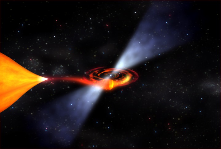
Seeking Gravitational Wave Sources
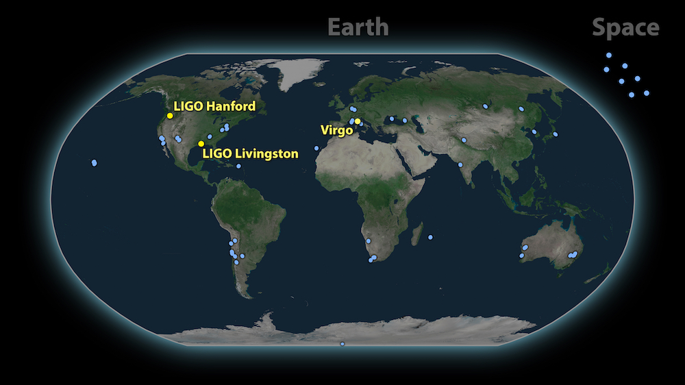
Locations of the observatories that followed up on the detection of the gravitational wave signal GW170817. Click to enlarge. [LIGO-Virgo]
Searches for gravitational wave sources are challenging because the search areas are often large, telescope time is limited, and the events are transient. How can we track down the causes of gravitational wave signals in a way that makes the most efficient use of the available observing time? In a recent publication, B. Parazin (Northeastern University and University of Minnesota) put a new observation-scheduling algorithm to the test.
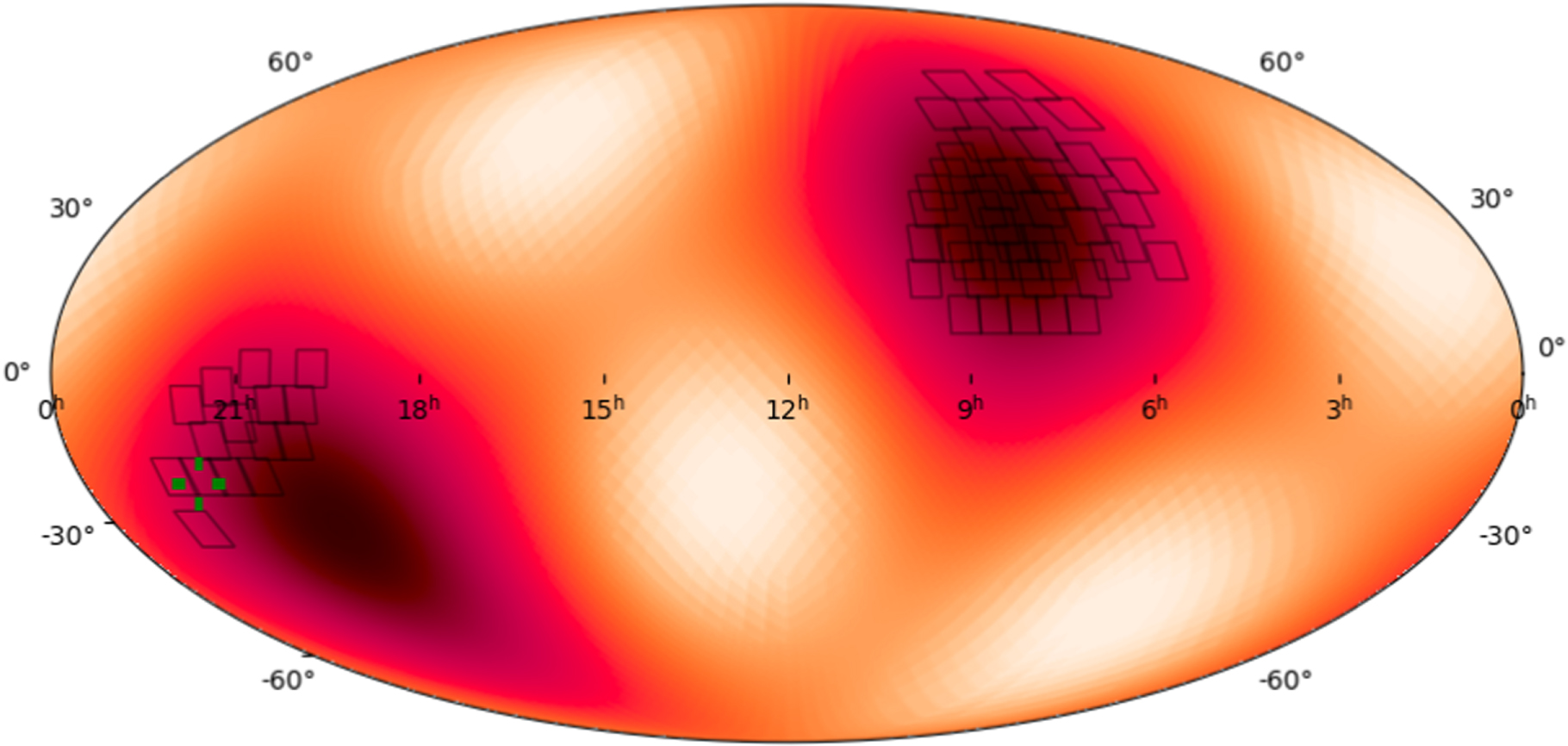
An example sky map in which the color scale indicates the probability density of the gravitational wave source’s location. The black shapes show the ZTF observing fields and the green crosshairs show the actual location of the event. [Parazin et al. 2022]
Scheduling Telescope Time
Parazin and collaborators tested a new algorithm optimized for the Zwicky Transient Facility (ZTF), which is designed to detect transient events. The team aimed to maximize the odds of tracking down the source of a new gravitational wave signal while minimizing the amount of observing time needed. They also accounted for factors that are unique to the ZTF, such as the time needed to switch between filters.
In addition to the particulars of the ZTF observing setup, the algorithm takes as an input a map of the sky showing the probable locations of a gravitational wave source, which is released by gravitational wave observatories when a new signal is detected. From there, the algorithm identifies which out of the ZTF telescope’s 1,778 possible pointing directions are appropriate, groups pointings that are continuously observable during a selected length of time, and orders the pointings within each group so as to minimize the amount of time the telescope spends between observations.
Improving Efficiency
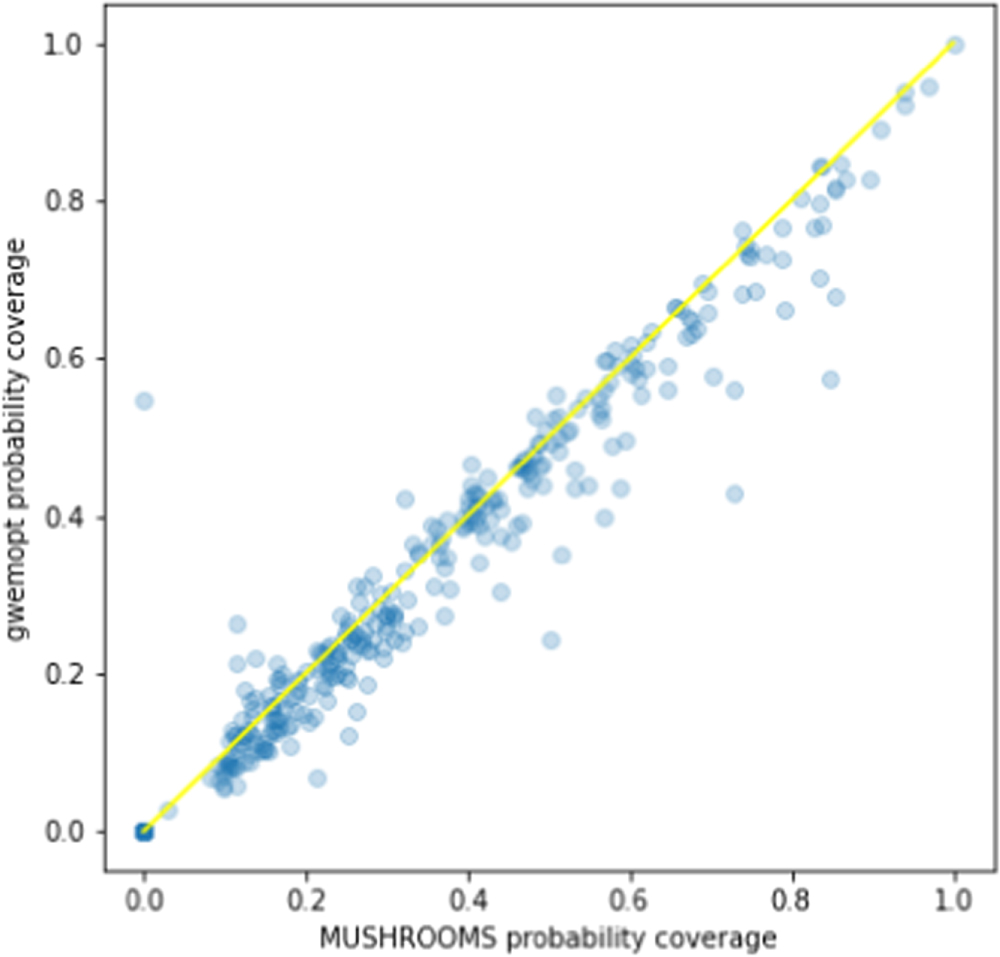
Comparison of the probability coverage of the existing algorithm in use by the ZTF (gwemopt) to that of the new algorithm introduced in this work (MUSHROOMS). The new algorithm performs better than the existing algorithm for cases located under the yellow line. [Parazin et al. 2022]
A final wrinkle is the fact that transient sources can fade rapidly, making the order in which the observations are carried out important — reach a source too late, and it may have dimmed beyond detection. When testing both algorithms on finding rapidly fading synthetic kilonovae, the team found that 1) once again, the hybrid approach had the best performance, and 2) the new algorithm had an advantage over the existing software when the search area was large.
While Parazin and collaborators stress that there are further improvements to be made, the algorithm in its current form shows promising improvements to our ability to track down the sources of gravitational waves.
Citation
“Foraging with MUSHROOMS: A Mixed-integer Linear Programming Scheduler for Multimessenger Target of Opportunity Searches with the Zwicky Transient Facility,” B. Parazin et al 2022 ApJ 935 87. doi:10.3847/1538-4357/ac7fa2


