Features RSS

NGC 3156

Observed “burps” from the shredding of stars by supermassive black holes suggest that this behavior is more common in an unusual type of galaxy. A new study has examined NGC 3156, an example from this galaxy type, to better understand what causes this preference.

Stellar Betrayal

TDE

An artist’s illustration of a tidal disruption event, in which a star is sent on a plunging orbit near a supermassive black hole and is subsequently torn apart by the black hole’s tidal forces. [NASA/CXC/M.Weiss]

Tidal disruption events (TDEs) are events where a star plunges too close to a supermassive black hole and is torn apart by the black hole’s tidal forces. We’ve observed roughly a dozen of these violent events in the last five years, and we expect to finds hundreds to thousands more with future surveys.

TDEs are triggered when a star is sent on a plunging orbit close to a supermassive black hole. But what sends the star into harm’s way? One possible culprit is a dynamical mechanism known as two-body relaxation. In this process, stars orbiting a black hole undergo individual star–star interactions that, with a close enough encounter, can send them on plunging orbits.

Choosing an Unusual Host

One puzzle with TDEs is that they tend to be preferentially found in rather unusual galaxies: galaxies that recently exhibited a lot of star formation but are now quiescent. In particular, several of the TDEs have been discovered in what are known as “E+A galaxies,” a rare subtype of elliptical galaxy that has recently undergone a major starburst.

Since this subtype makes up only ~0.1% of all galaxies, it’s surprising that we’ve found so many TDEs in E+A galaxies so far. So why the preference?

In an effort to answer this question, two scientists, Nicholas Stone (Einstein Fellow at Columbia University) and Sjoert van Velzen (Hubble Fellow at Johns Hopkins University), have teamed up to examine a nearby E+A galaxy, NGC 3156.

TDE rates

Tidal disruption rates as a function of central supermassive-black-hole mass. The blue curve shows the authors’ model for NGC 3156 (assuming different masses for its central black hole), and the black curve shows the power-law best fit for a large galaxy sample. NGC 3156’s predicted TDE rate is an order of magnitude higher that of a typical galaxy. [Stone & van Velzen 2016]

Collisions in a Crowded Nucleus

By analyzing Hubble Space Telescope photometry of NGC 3156, Stone and van Velzen determine that there is an overdensity of stars in the central region of the galaxy — which is expected to be the case for all E+A galaxies, due to their starburst history. The authors next use their measurements and arguments of stellar density and dynamics to calculate a predicted rate of two-body star–star interactions that lead to TDEs.

Stone and van Velzen predict that TDEs from two-body interactions should occur at a rate of ~10-3 per year in NGC 3156. This is an order of magnitude larger than the rate that the same calculations would predict for a typical galaxy (10-4 per year).

The authors’ observations and analysis of NGC 3156 strongly support the idea that E+A galaxies overproduce TDEs because their very dense centers — created by past starbursts — provide a highly collisional environment, allowing more star–star interactions. These interactions can then lead to stellar orbits that plunge near the supermassive black hole at the galactic center, producing TDEs.

Citation

Nicholas C. Stone and Sjoert van Velzen 2016 ApJ 825 L14. doi:10.3847/2041-8205/825/1/L14

Magellanic System

Recent deep observations of the Large Magellanic Cloud (LMC), a satellite galaxy of the Milky Way, have revealed a faint arc of stars extending from its northern outskirts. Was this stream created by the gravitational pull of the Milky Way? Or could it have a more violent source?

LMC outskirts

The area surrounding the LMC. The stellar arc discovered with the Dark Energy Survey is shown in the region labeled A. The current study discovered additional asymmetric substructure in the region labeled C. [Besla et al. 2016]

Searching for Spiral Structure

When deep optical imaging by the Dark Energy Survey discovered this faint stream of stars extending eastward from the northern periphery of the LMC, scientists’ assumption was that this arm was created by the tidal pull of the Milky Way.

But a team of authors led by Gurtina Besla (University of Arizona) argue for an alternate theory: what if this stellar stream was instead caused by repeated interactions between the LMC and the Small Magellanic Cloud (SMC)?

One way to test these models is to look for a symmetrically corresponding arm in the south of the LMC extending west; such an arm would be expected if tidal forces from the Milky Way were acting globally on the LMC to create the northeast arm.

The Dark Energy Survey’s footprint doesn’t cover the southern regions of the LMC’s disk, but Besla and collaborators have an alternative: they performed their own wide-field survey using small robotic telescopes, which provide long exposures at low cost.

Modeling Past and Future Interactions

Interaction simulations

The simulated interaction history of the LMC and SMC in isolation (i.e., without the Milky Way). The top left panel shows the SMC–LMC separation as a function of time; the remaining panels show the system at different stages of the simulation. Only particles associated with the LMC are shown here; the SMC’s position is indicated by a blue star. [Besla et al. 2016]

The team’s deep optical observations of the LMC and SMC fields confirmed the presence of asymmetric stellar arc structures in the northern outskirts of the LMC — and they didn’t find any corresponding structures in the southern region. This strongly supports the idea that the structures were caused by interactions between the LMC and the SMC, rather than by galactic tides.

To further test this model, Besla and collaborators ran a series of simulations of interactions between LMC and SMC, first in isolation and then with the added tidal forces from the Milky Way.

The simulations supported the conclusions drawn from the observations: while Milky Way tides may influence the final distribution of structures in the LMC’s outskirts, close interactions between the LMC and the SMC appear to be the primary cause responsible for the asymmetric spiral structure found.

As is shown in the authors’ simulations, the complete model of LMC/SMC interactions predicts that the two dwarfs will continue to interact until they eventually merge. Comparison of detailed simulations with future high-resolution observations of the LMC should help us further understand the interaction history of the LMC and SMC, thereby allowing us to better predict their eventual fate.

Bonus

Check out the gif below, cut from a video of the authors’ simulations. In these simulations, the SMC interacts with the LMC over the span of ~9 Gyr, passing through it several times before the LMC completely cannibalizes the SMC. You can visit the authors’ article to view the original video.

LMC-SMC simulation

Citation

Gurtina Besla et al 2016 ApJ 825 20. doi:10.3847/0004-637X/825/1/20

Carina nebula

Can protoplanetary disks form and be maintained around low-mass stars in the harsh environment of a highly active, star-forming nebula? A recent study examines the Carina nebula to answer this question.

Crowded Clusters

Stars are often born in clusters that contain both massive and low-mass stars. The most massive stars in these clusters emit far-ultraviolet and extreme-ultraviolet light that irradiates the region around them, turning the surrounding area into a hostile environment for potential planet formation.

Planet formation from protoplanetary disks typically requires timescales of at least 1–2 million years. Could the harsh radiation from massive stars destroy the protoplanetary disks around low-mass stars by photoevaporation before planets even have a chance to form?

protoplanetary disk

Artist’s impression of a protoplanetary disk. Such disks can be photoevaporated by harsh ultraviolet light from nearby massive stars, causing the disk to be destroyed before planets have a chance to form within them. [ESO/L. Calçada]

Turning ALMA Toward Carina

A perfect case study for exploring hostile environments is the Carina nebula, located about 7500 lightyears away — and home to nearly 100 O-type stars as well as tens of thousands of lower-mass young stars. The Carina population is ~1–4 Myr old: old enough to form planets within protoplanetary disks, but also old enough that photoevaporation could already have wreaked havoc on those disks.

Due to the dense stellar populations in Carina’s clusters, this is a difficult region to explore, but the Atacama Large Millimeter-submillimeter Array (ALMA) is up to the task. In a recent study, a team of scientists led by Adal Mesa-Delgado (Pontifical Catholic University of Chile) made use of ALMA’s high spatial resolution to image four regions spaced throughout Carina, searching for protoplanetary disks.

Detections and Non-Detections

Disk detections

Two evaporating gas globules in the Carina nebula, 104-593 and 105-600, that each contain a protoplanetary disk. The top panels are Hubble images of the globules; the bottom panels are ALMA images of the disks detected within them. [Mesa-Delgado et al. 2016]

In searching regions outside of the densest, most luminous clusters, the team succeeded in detecting two protoplanetary disks. This region in Carina now marks the most distant massive cluster in which disks have ever been imaged! The discovered disks have radii of roughly 60 AU and masses of 30 and 50 Jupiter masses — and given their ages, it’s entirely plausible that planets are actively forming in these disks.

Equally important: Mesa-Delgado and collaborators failed to detect any indication of disks in the core of Trumpler 14, a cluster in Carina that is home to some of the most massive and luminous stars in the Galaxy. This non-detection suggests that the particularly harsh environment of Trumpler 14 is too brutal for disks within it to survive.

These observations provide new clues as to where we should be looking to study planet formation: less dense regions in star-forming nebulae seem to be locations that can support giant-planet-forming disks, whereas the harsh radiation fields of especially dense subclusters seem to cause the rapid destruction of such disks.

Citation

A. Mesa-Delgado et al 2016 ApJ 825 L16. doi:10.3847/2041-8205/825/1/L16

persistence map

Coronal dimming

This time series of SDO images of an active region shows coronal dimming as well as flares. These images can be combined into a minimum-value persistence map (bottom panel) that better reveals the entire dimming region. [Adapted from Thompson & Young 2016]

What if there were a better way to analyze a comet’s tail, the dimming of the Sun’s surface, or the path of material in a bright solar eruption? A recent study examines a new technique for looking at these evolving features.

Mapping Evolving Features

Sometimes interesting advances in astronomy come from simple, creative new approaches to analyzing old data. Such is the case in a new study by Barbara Thompson and Alex Young (NASA Goddard Space Flight Center), which introduces a technique called “persistence mapping” to better examine solar phenomena whose dynamic natures make them difficult to analyze.

What is a persistence map? Suppose you have a set of N images of the same spatial region, with each image taken at a different time. To create a persistence map of these images, you would combine this set of images by retaining only the most extreme (for example, the maximum) value for each pixel, throwing away the remaining N-1 values for each pixel.

Persistence mapping is especially useful for bringing out rare or intermittent phenomena — features that would often be washed out if the images were combined in a sum or average instead. Thompson and Young describe three example cases where persistence mapping brings something new to the table.

Comet Lovejoy

Top: Single SDO image of Comet Lovejoy. Center: 17 minutes of SDO images, combined in a persistence map. The structure of the tail is now clearly visible. Bottom: For comparison, the average pixel value for this sequence of images. Click for a closer look! [Thompson & Young 2016]

A Comet’s Tail

As Comet Lovejoy passed through the solar corona in 2011, solar physicists analyzed extreme ultraviolet images of its tail — because the motion of the tail particles reveals information about the local coronal magnetic field.

Past analyses have averaged or summed images of the comet in orbit to examine its tail. But a persistence map of the maximum pixel values far more clearly shows the striations within the tail that reveal the directions of the local magnetic field lines.

Dimming of the Sun

Dimming of the Sun’s corona near active regions tells us about the material that’s evacuated during coronal mass ejections. This process can be complex: regions dim at different times, and flares sometimes hide the dimming, making it difficult to observe. But understanding the entire dimming region is necessary to infer the total mass loss and complete magnetic footprint of a gradual eruption from the Sun’s surface.

Erupting prominence

SDO and STEREO-A images of a prominence eruption. Tracking the falling material is difficult due to the complex background. [Thompson & Young 2016]

Creating a persistence map of minimum pixel values achieves this — and also neatly sidesteps the problem of flares hiding the dimming regions, since the bright pixels are discarded. In the authors’ example, a persistence map estimates 50% more mass loss for a coronal dimming event than the traditional image analysis method, and it reveals connections between dimming regions that were previously missed.

An Erupting Prominence

The authors’ final example is of falling prominence material after a solar eruption, seen in absorption against the bright corona. They show that you can construct a persistence map of minimum pixel values over the time the material falls (see the cover image), allowing the material’s paths to be tracked despite the evolving background behind it. Tracing these trajectories provides information about the local magnetic field.

Thompson and Young’s examples indicate that persistence mapping clearly provides new information in some cases of intermittent or slowly evolving solar phenomena. It will be interesting to see where else this technique can be applied!

Citation

B. J. Thompson and C. A. Young 2016 ApJ 825 27. doi:10.3847/0004-637X/825/1/27

Spiral protoplanetary disk

What causes the large-scale spiral structures found in some protoplanetary disks? Most models assume they’re created by newly-forming planets, but a new study suggests that planets might have nothing to do with it.

Perturbations from Planets?

In some transition disks — protoplanetary disks with gaps in their inner regions — we’ve directly imaged large-scale spiral arms. Many theories currently attribute the formation of these structures to young planets: either the direct perturbations of a planet embedded in the disk cause the spirals, or they’re indirectly caused by the orbit of a planetary body outside of the arms.

MWC 758

Another example of spiral arms detected in a protoplanetary disk, MWC 758. [NASA/ESA/ESO/M. Benisty et al.]

But what if you could get spirals without any planets? A team of scientists led by Matías Montesinos (University of Chile) have recently published a study in which they examine what happens to a shadowed protoplanetary disk.

Casting Shadows with Warps

In the team’s setup, they envision a protoplanetary disk that is warped: the inner region is slightly tilted relative to the outer region. As the central star casts light out over its protoplanetary disk, this disk warping would cause some regions of the disk to be shaded in a way that isn’t axially symmetric — with potentially interesting implications.

Montesinos and collaborators ran 2D hydrodynamics simulations to determine what happens to the motion of particles within the disk when they pass in and out of the shadowed regions. Since the shadowed regions are significantly colder than the illuminated disk, the pressure in these regions is much lower. Particles are therefore accelerated and decelerated as they pass through these regions, and the lack of axial symmetry causes spiral density waves to form in the disk as a result.

initial shadow profile

Initial profile for the stellar heating rate per unit area for one of the authors’ simulations. The regions shadowed as a result of the disk warp subtend 0.5 radians each (shown on the left and right sides of the disks here). [Montesinos et al. 2016]

Observations of Shadow Spirals

In the authors’ models, two shadowed regions result in the formation of two spiral arms. The arms that develop start at a pitch angle of 15°–22°, and gradually evolve to a shallower 11°–14° pitch at distances of ~65–150 AU.

The more luminous the central star, the more quickly the spiral arms form, due to the greater contrast between illuminated and shadowed disk regions: for a 0.25 solar-mass disk illuminated by a 1 solar-luminosity star, arms start to form after about 2500 orbits. If we increase the star’s brightness to 100 solar luminosities, the arms form after only 150 orbits.

Montesinos and collaborators conclude by testing whether or not such spiral structures would be observable. They use a 3D radiative transfer code to produce scattered-light predictions of what the disk would look like to direct-imaging telescopes. They find that these shadow-induced spirals should be detectable.

This first study clearly demonstrates that large-scale spiral density waves can form in protoplanetary disks without the presence of planets. The authors now plan to add more detailed physics to their models to better understand what we might observe when looking at systems that were shaped in this way.

disk density evolution

Density evolution in two shadowed disks. Top row: disk illuminated by a 100 L⊙ star, at 150, 250, and 500 orbits (from left to right). Bottom row: disk illuminated by a 1 L⊙ star, at 2500, 3500, and 4000 orbits. The rightmost top and bottom panels show control simulations (no shadows were present on the disk) after 1000 and 6000 orbits. (A different type of spiral starts to develop in the bottom control simulation as a result of a gravitational instability, but it never extends to the edges of the disk.) [Montesinos et al. 2016]

Citation

Matías Montesinos et al 2016 ApJ 823 L8. doi:10.3847/2041-8205/823/1/L8

cosmic rays

In a cubic kilometer of volume of ice under Antarctica, an observatory called IceCube is taking measurements that may help us to determine what causes the ultra-high-energy cosmic rays (UHECRs) we occasionally observe from Earth. A recent study reports on its latest results.

Atomic Baseballs

Cosmic rays are high-energy radiation primarily composed of protons and atomic nuclei. When these charged and extremely energetic particles impact the Earth’s atmosphere on their journey through space, they generate showers of secondary particles that we then detect.

A UHECR is any cosmic-ray particle with a kinetic energy exceeding 1018 eV — and some have been detected with energies of more than 1020 eV! In practical terms, this is an atomic nucleus with the same kinetic energy as a baseball pitched at 60mph. These unbelievably energetic particles are quite rare, but we’ve observed them for decades. Yet in spite of this, the source of UHECRs is unknown.

GRB

Illustration of a gamma-ray burst in a star-forming region. Could these phenomena accelerate UHECRs to their enormous energies? [NASA/Swift/Mary Pat Hrybyk-Keith and John Jones]

Gamma-Ray Burst Fireballs

One proposed source that could accelerate particles to these energies is a gamma-ray burst (GRB). In some models for GRBs, the explosion is envisioned as a relativistically expanding fireball of electrons, photons and protons. Internal shock fronts accelerate electrons and protons within the fireball, generating UHECRs, gamma rays, and neutrinos in the process.

Because the charged cosmic-ray particles can be easily deflected as they travel, it’s difficult to identify where they came from. Neutrinos and photons, on the other hand, both travel largely undeflected through the universe. As a result, if we detect high-energy neutrinos that are correlated with gamma-ray photons from a GRB, this would provide strong support for GRB fireball models for UHECR production.

Heading Under the Ice

IceCube

The IceCube Laboratory in Antarctica. Beneath the Antarctic ice lie more than 5,000 detectors over a cubic kilometer of volume. [IceCube/NSF/S. Lidstrom]

How do we search for these neutrinos? Enter IceCube, an neutrino observatory that consists of a cubic kilometer of detectors lying deep under the Antarctic ice. This observatory is designed to detect the by-products of the rare interactions neutrinos passing through the Earth might have with molecules of water in the ice.

In a recently published study by the IceCube Collaboration, the team performed a three-year search for neutrinos that were correlated with the locations and times of more than 800 known GRBs during that period.

GRB fireball models

Three different fireball models for GRBs, and the predicted neutrino flux from each. The neutrinos potentially detectable by IceCube are shown with solid segments. IceCube’s detections (and lack thereof) place new constraints on these models. [Aartsen et al. 2016]

New Constraints

From three years of data, the collaboration reports the detection of five low-significance events correlated with five GRBs. But these events are also consistent with the background of charged particles generated in Earth’s atmosphere. What does this mean? These detections could indicate a small number of real neutrinos generated by GRBs — or they could just be background noise.

Either way, these results from IceCube provide a new upper limit on the association of neutrinos with gamma-ray bursts. This constrains which production mechanisms are possible, eliminating some models for UHECR acceleration by GRB fireballs.

What’s next? The collaboration indicates that the next generation IceCube-Gen2 detector, planned for the future, will be even more sensitive — which will either result in the detection of more subtle neutrino events associated with GRBs, or it will further disfavor GRBs as the production mechanism for UHECRs.

Citation

M. G. Aartsen et al 2016 ApJ 824 115. doi:10.3847/0004-637X/824/2/115

LMC hypervelocity star

How are the hypervelocity stars we’ve observed in our galaxy produced? A recent study suggests that these escapees could be accelerated by a massive black hole in the center of the Large Magellanic Cloud.

A Black Hole Slingshot

Since their discovery in 2005, we’ve observed dozens of candidate “hypervelocity stars” — stars whose velocity in the rest frame of our galaxy exceeds the local escape velocity of the Milky Way. These stars present a huge puzzle: how did they attain these enormous velocities?

One potential explanation is known as the Hills mechanism. In this process, a stellar binary is disrupted by a close encounter with a massive black hole (like those thought to reside at the center of every galaxy). One member of the binary is flung out of the system as a result of the close encounter, potentially reaching very large velocities.

LHA 120-N 11

A star-forming region known as LHA 120-N 11, located within the LMC. Some binary star systems within the LMC might experience close encounters with a possible massive black hole at the LMC’s center. [ESA/NASA/Hubble]

Blame the LMC?

Usually, discussions of the Hills mechanism assume that Sagittarius A*, the supermassive black hole at the center of the Milky Way, is the object guilty of accelerating the hypervelocity stars we’ve observed. But what if the culprit isn’t Sgr A*, but a massive black hole at the center of the Large Magellanic Cloud (LMC), one of the Milky Way’s satellite galaxies?

Though we don’t yet have evidence of a massive black hole at the center of the LMC, the dwarf galaxy is large enough to potentially host one as large as 100,000 solar masses. Assuming that it does, two scientists at the University of Cambridge, Douglas Boubert and Wyn Evans, have now modeled how this black hole might tear apart binary star systems and fling hypervelocity stars around the Milky Way.

Models for Acceleration

Boubert and Evans determined that the LMC’s hypothetical black hole could easily eject stars at ~100 km/s, which is the escape velocity of the LMC. When this speed is combined with the orbital velocity of the LMC itself (another ~380 km/s relative to the Milky Way), this could result in hypervelocity stars moving faster than the escape speed of the Milky Way, as observed.

HVS distribution

Predicted distribution of hypervelocity stars ejected from the LMC, in galactic coordinates. The red crosses show locations of detected hypervelocity stars, and the green arrow marks the path of the LMC over the last 350 million years. [Boubert & Evans 2016]

If the LMC is indeed ejecting hypervelocity stars along its orbit, this could explain an observed anisotropy in the hypervelocity stars we’ve detected, with many of these stars clustering in the constellations of Leo and Sextans. This clustering is consistent with stars ejected ahead of the LMC’s orbit.

How can we test this model for the production of hypervelocity stars? The authors’ model predicts the presence of a significant number of hypervelocity stars near the LMC in the southern hemisphere, a region which has been poorly surveyed before now. Surveys such as SkyMapper and Gaia, however, will observe this region — and their discoveries (or lack thereof) should provide a useful test of whether hypervelocity stars are accelerated by the LMC.

Citation

Douglas Boubert and N. Wyn Evans 2016 ApJ 825 L6. doi:10.3847/2041-8205/825/1/L6

Planet Nine orbit

What’s the news coming from the research world on the search for Planet Nine? Read on for an update from a few of the latest studies.

Planet Nine

Artist’s illustration of Planet Nine, a hypothesized Neptune-sized planet orbiting in the distant reaches of our solar system. [Caltech/Robert Hurt]

What is Planet Nine?

In January of this year, Caltech researchers Konstantin Batygin and Mike Brown presented evidence of a distant ninth planet in our solar system. They predicted this planet to be of a mass and volume consistent with a super-Earth, orbiting on a highly eccentric path with a period of tens of thousands of years.

Since Batygin and Brown’s prediction, scientists have been hunting for further signs of Planet Nine. Though we haven’t yet discovered an object matching its description, we have come up with new strategies for finding it, we set some constraints on where it might be, and we made some interesting theoretical predictions about its properties.

Resonant Orbits

Visualizations of the resonant orbits of the four longest-period Kuiper belt objects, depicted in a frame rotating with the mean angular velocity of Planet Nine. Planet Nine’s position is on the right (with the trace of possible eccentric orbits e=0.17 and e=0.4 indicated in red). [Malhotra et al 2016]

Here are some of the newest constraints on Planet Nine from studies published just within the past two weeks.

Resonant Orbits

Renu Malhotra (University of Arizona’s Lunar and Planetary Laboratory) and collaborators present further evidence of  the shaping of solar system orbits by the hypothetical Planet Nine. The authors point out that the four longest-period Kuiper belt objects (KBOs) have orbital periods close to integer ratios with each other. Could it be that these outer KBOs have become locked into resonant orbits with a distant, massive body?

The authors find that a distant planet orbiting with a period of ~17,117 years and a semimajor axis ~665 AU would have N/1 and N/2 period ratios with these four objects. If this is correct, it significantly constrains the parameters of Planet Nine’s orbit — as well as where it currently could be within its orbit.

Eliminating Hiding Spots

Brown and Batygin have returned, this time with more detailed estimates of Planet Nine’s potential orbit and location. By performing an enormous suite of simulations and then comparing the outcomes to actual observations of the distribution of KBOs, the authors narrow the allowed range for Planet Nine’s orbital characteristics.

Where to look for Planet Nine

Authors’ predictions for the location, distance, brightness, and speed of Planet Nine throughout its orbit. Colored regions have been or will be explored by previous or current surveys capable of detecting the planet. Black regions remain places where Planet Nine could lurk. [Brown & Batygin 2016]

Brown and Batygin find that the allowed orbits for Planet Nine have perihelia of ~150–350 AU, semimajor axes of ~380–980 AU, and masses of ~5–20 Earth masses. Using these values and what we know about detection limits of previous and current surveys, we can rule out roughly two thirds of Planet Nine’s orbit, narrowing its position to be somewhere near aphelion.

Planet Nine’s Atmosphere

Finally, Jonathan Fortney (UC Santa Cruz) and collaborators model Planet Nine’s atmosphere. Rather than assuming the planet behaves like a blackbody, they use the planet’s predicted orbit — as well as a range of plausible masses and interior structures — in models that treat the body like the giant planets of our solar system.

The authors find Planet Nine is likely quite cold, as expected, with an effective temperature of ~35–50 K at most (for reference, Neptune is around 60 K). Because of this cool temperature, the authors speculate that methane may condense out of the atmosphere, changing the planet’s reflection and emission spectra. This would cause the planet to appear much “bluer” than planets like Uranus and Neptune in infrared energy bands.

The constraints from these studies continue to support the existence of Planet Nine, narrow down the regions in which we should search for it, and help us to better understand what signatures we’re looking for. In the words of Fortney et al., “Let the hunt continue.”

Citation

Renu Malhotra et al 2016 ApJ 824 L22. doi:10.3847/2041-8205/824/2/L22
Michael E. Brown and Konstantin Batygin 2016 ApJ 824 L23. doi:10.3847/2041-8205/824/2/L23
Jonathan J. Fortney et al 2016 ApJ 824 L25. doi:10.3847/2041-8205/824/2/L25

NEO

How can we hunt down all the near-Earth asteroids that are capable of posing a threat to us? A new study looks at whether the upcoming Large Synoptic Survey Telescope (LSST) is up to the job.

Charting Nearby Threats

LSST is an 8.4-m wide-survey telescope currently being built in Chile. When it goes online in 2022, it will spend the next ten years surveying our sky, mapping tens of billions of stars and galaxies, searching for signatures of dark energy and dark matter, and hunting for transient optical events like novae and supernovae. But in its scanning, LSST will also be looking for asteroids that approach near Earth.

NEOs discovered

Cumulative number of near-Earth asteroids discovered over time, as of June 16, 2016. [NASA/JPL/Chamberlin]

Near-Earth objects (NEOs) have the potential to be hazardous if they cross Earth’s path and are large enough to do significant damage when they impact Earth. Earth’s history is riddled with dangerous asteroid encounters, including the recent Chelyabinsk airburst in 2013, the encounter that caused the kilometer-sized Meteor Crater in Arizona, and the impact thought to contribute to the extinction of the dinosaurs.

Recognizing the potential danger that NEOs can pose to Earth, Congress has tasked NASA with tracking down 90% of NEOs larger than 140 meters in diameter. With our current survey capabilities, we believe we’ve discovered roughly 25% of these NEOs thus far. Now a new study led by Tommy Grav (Planetary Science Institute) examines whether LSST will be able to complete this task.

absolute magnitudes of NEOs

Absolute magnitude, H, of a synthetic NEO population. Though these NEOs are all larger than 140 m, they have a large spread in albedos. [Grav et al. 2016]

Can LSST Help?

Based on previous observations of NEOs and resulting predictions for NEO properties and orbits, Grav and collaborators simulate a synthetic population of NEOs all above 140 m in size. With these improved population models, they demonstrate that the common tactic of using an asteroid’s absolute magnitude as a proxy for its size is a poor approximation, due to asteroids’ large spread in albedos. Roughly 23% of NEOs larger than 140 m have absolute magnitudes fainter than H = 22 mag, the authors show — which is the value usually assumed as the default absolute magnitude of a 140 m NEO.

NEO fraction detectable

Fraction of NEOs we’ve detected as a function of time based on the authors’ simulations of the current surveys (red), LSST plus the current surveys (black), NEOCam plus the current surveys (blue), and the combined result for all surveys (green). [Grav et al. 2016]

Taking this into account, Grav and collaborators then use information about the planned LSST survey strategies and detection limits to test what fraction of this synthetic NEO population LSST will be able to detect in its proposed 10-year mission.

The authors find that, within 10 years, LSST will likely be able to detect only 63% of NEOs larger than 140 m. Luckily, LSST may not have to work alone; in addition to the current surveys in operation, a proposed infrared space-based survey mission called NEOCam is planned for launch in 2021. If NEOCam is funded, it will complement LSST’s discovery capabilities, potentially allowing the two surveys to jointly achieve the 90% detection goal within a decade.

Citation

T. Grav et al 2016 AJ 151 172. doi:10.3847/0004-6256/151/6/172

Jet launch after merger

With the recent discovery of gravitational waves from the merger of two black holes, it’s especially important to understand the electromagnetic signals resulting from mergers of compact objects. New simulations successfully follow a merger of two neutron stars that produces a short burst of energy via a jet consistent with short gamma-ray burst (sGRB) detections.

neutron stars

Still from the authors’ simulation showing the two neutron stars, and their magnetic fields, before merger. [Adapted from Ruiz et al. 2016]

Challenging System

We have long suspected that sGRBs are produced by the mergers of compact objects, but this model has been difficult to prove. One major hitch is that modeling the process of merger and sGRB launch is very difficult, due to the fact that these extreme systems involve magnetic fields, fluids and full general relativity.

Traditionally, simulations are only able to track such mergers over short periods of time. But in a recent study, Milton Ruiz (University of Illinois at Urbana-Champaign and Industrial University of Santander, Colombia) and coauthors Ryan Lang, Vasileios Paschalidis and Stuart Shapiro have modeled a binary neutron star system all the way through the process of inspiral, merger, and the launch of a jet.

A Merger Timeline

How does this happen? Let’s walk through one of the team’s simulations, in which dipole magnetic field lines thread through the interior of each neutron star and extend beyond its surface (like magnetic fields found in pulsars). In this example,  the two neutron stars each have a mass of 1.625 solar masses.

  1. Simulation start (0 ms)
    Loss of energy via gravitational waves cause the neutron stars to inspiral.
  2. Merger (3.5 ms)
    The neutron stars are stretched by tidal effects and make contact. Their merger produces a hypermassive neutron star that is supported against collapse by its differential (nonuniform) rotation.
  3. Delayed collapse into a black hole (21.5 ms)
    Once the differential rotation is redistributed by magnetic fields and partially radiated away in gravitational waves, the hypermassive neutron star loses its support and collapses to a black hole.
  4. Plasma velocities turn around (51.5 ms)
    Initially the plasma was falling inward, but as the disk of neutron-star debris is accreted onto the black hole, energy is released. This turns the plasma near the black hole poles around and flings it outward.
  5. Magnetic field forms a helical funnel (62.5 ms)
    The fields near the poles of the black hole amplify as they are wound around, creating a funnel that provides the wall of the jet.
  6. Jet outflow extends to heights greater than 445 km (64.5 ms)
  7. The disk is all accreted and, since the fuel is exhausted, the outflow shuts off (within 100ms)

Neutron-Star Success

GW signature

Plot showing the gravitational wave signature for one of the authors’ simulations. The moments of merger of the neutron stars and collapse to a black hole are marked. [Adapted from Ruiz et al. 2016]

These simulations show that no initial black hole is needed to launch outflows; a merger of two neutron stars can result in an sGRB-like jet. Another interesting result is that the magnetic field configuration doesn’t affect the formation of a jet: neutron stars with magnetic fields confined to their interiors launch jets as effectively as those with pulsar-like magnetic fields. The accretion timescale for both cases is consistent with the duration of an sGRB.

While this simulation models milliseconds of real time, it’s enormously computationally challenging and takes months to simulate. The successes of this simulation represent exciting advances in numerical relativity, as well as in our understanding of the electromagnetic counterparts that may accompany gravitational waves.

Bonus

Check out this awesome video of the authors’ simulations. The colors differentiate the plasma density and the white lines depict the pulsar-like magnetic field that initially threads the two merging neutron stars. Watch as the neutron stars evolve through the different stages outlined above, eventually forming a black hole and launching a powerful jet. [Simulations and visualization by M. Ruiz, R. Lang, V. Paschalidis, S. Shapiro and the Illinois Relativity Group REU team: S. Connelly, C. Fan, A. Khan, and P. Wongsutthikoson]

Citation

Milton Ruiz et al 2016 ApJ 824 L6. doi:10.3847/2041-8205/824/1/L6


1 108 109 110 111 112 122